"Spread in model climate sensitivity traced to atmospheric convective mixing," by S. C. Sherwood, S. Bony & J.-L. Dufresne, Nature 505 (2014); doi: 10.1038/nature12829

Nature, 505 (2 January 2014) 37-42; doi: 10.1038/nature12829

Spread in model climate sensitivity traced to atmospheric convective mixing

• Steven C. Sherwood,
• Sandrine Bony and
•  Jean-Louis Dufresne

Abstract

Equilibrium climate sensitivity refers to the ultimate change in global mean temperature in response to a change in external forcing. Despite decades of research attempting to narrow uncertainties, equilibrium climate sensitivity estimates from climate models still span roughly 1.5 to 5 degrees Celsius for a doubling of atmospheric carbon dioxide concentration, precluding accurate projections of future climate. The spread arises largely from differences in the feedback from low clouds, for reasons not yet understood. Here we show that differences in the simulated strength of convective mixing between the lower and middle tropical troposphere explain about half of the variance in climate sensitivity estimated by 43 climate models. The apparent mechanism is that such mixing dehydrates the low-cloud layer at a rate that increases as the climate warms, and this rate of increase depends on the initial mixing strength, linking the mixing to cloud feedback. The mixing inferred from observations appears to be sufficiently strong to imply a climate sensitivity of more than 3 degrees for a doubling of carbon dioxide. This is significantly higher than the currently accepted lower bound of 1.5 degrees, thereby constraining model projections towards relatively severe future warming.

See 10 figures at this link:  http://www.nature.com/nature/journal/v505/n7481/full/nature12829.html

Planet likely to warm by 4C by 2100, scientists warn

New climate model taking greater account of cloud changes indicates heating will be at higher end of expectations

by Damian Carrington, The Guardian, December 31, 2013

The role clouds play in climate change has been something of a mystery – until now. Photograph: Frank Rumpenhorst/ Frank Rumpenhorst/dpa/Corbis

Temperature rises resulting from unchecked climate change will be at the severe end of those projected, according to a new scientific study.

The scientist leading the research said that unless emissions of greenhouse gases were cut, the planet would heat up by a minimum of 4 degrees centigrade by 2100, twice the level the world's governments deem dangerous.

The research indicates that fewer clouds form as the planet warms, meaning less sunlight is reflected back into space, driving temperatures up further still. The way clouds affect global warming has been the biggest mystery surrounding future climate change.

Professor Steven Sherwood, at the University of New South Wales, in Australia, who led the new work, said: "This study breaks new ground twice: first by identifying what is controlling the cloud changes and second by strongly discounting the lowest estimates of future global warming in favour of the higher and more damaging estimates."

"4 C would likely be catastrophic rather than simply dangerous," Sherwood told the Guardian. "For example, it would make life difficult, if not impossible, in much of the tropics, and would guarantee the eventual melting of the Greenland ice sheet and some of the Antarctic ice sheet," with sea levels rising by many metres as a result.

The research is a "big advance" that halves the uncertainty about how much warming is caused by rises in carbon emissions, according to scientists commenting on the study, published in the journal Nature. Hideo Shiogama and Tomoo Ogura, at Japan's National Institute for Environmental Studies, said the explanation of how fewer clouds form as the world warms was "convincing," and agreed this indicated future climate would be greater than expected. But they said more challenges lay ahead to narrow down further the projections of future temperatures.

Scientists measure the sensitivity of the Earth's climate to greenhouse gases by estimating the temperature rise that would be caused by a doubling of CO2 in the atmosphere compared with pre-industrial levels – as is likely to happen within 50 years, on current trends. For two decades, those estimates have run from 1.5 to 5 C, a wide range; the new research narrowed that range to between 3 and 5 C, by closely examining the biggest cause of uncertainty: clouds.

The key was to ensure that the way clouds form in the real world was accurately represented in computer climate models, which are the only tool researchers have to predict future temperatures. When water evaporates from the oceans, the vapour can rise over 9 miles to form rain clouds that reflect sunlight; or it may rise just a few miles and drift back down without forming clouds. In reality, both processes occur, and climate models encompassing this complexity predicted significantly higher future temperatures than those only including the 9-mile-high clouds.

"Climate sceptics like to criticise climate models for getting things wrong, and we are the first to admit they are not perfect," said Sherwood. "But what we are finding is that the mistakes are being made by the models which predict less warming, not those that predict more."

He added: "Sceptics may also point to the 'hiatus' of temperatures since the end of the 20th century, but there is increasing evidence that this inaptly named hiatus is not seen in other measures of the climate system, and is almost certainly temporary."

Global average air temperatures have increased relatively slowly since a high point in 1998 caused by the ocean phenomenon El Niño, but observations show that heat is continuing to be trapped in increasing amounts by greenhouse gases, with over 90% disappearing into the oceans. Furthermore, a study in November suggested the "pause" may be largely an illusion resulting from the lack of temperature readings from polar regions, where warming is greatest.

Sherwood accepts his team's work on the role of clouds cannot definitively rule out that future temperature rises will lie at the lower end of projections. "But," he said, for that to be the case, "one would need to invoke some new dimension to the problem involving a major missing ingredient for which we currently have no evidence. Such a thing is not out of the question but requires a lot of faith."

He added: "Rises in global average temperatures of [at least 4 C by 2100] will have profound impacts on the world and the economies of many countries, if we don't urgently start to curb our emissions."

http://www.theguardian.com/environment/2013/dec/31/planet-will-warm-4c-2100-climate

David Spratt: Confused about the new IPCC's carbon budget? So am I.

by David Spratt, Climate Code Red, October 17, 2013

When the IPCC's new report on the physical basis of climate change was released in late September, media attention focused on a conclusion from the Summary for Policymakers that the world had emitted just over half of the allowable emissions if global warming is to be kept to 2 degrees Celsius (2 °C) of warming.

Unfortunately, because many people think if you have a budget you should spend every last dollar, the "carbon budget" message could be interpreted as saying there is plenty of budget left to spend. The respected climate researcher Ken Caldeira told Climate Progress that the carbon budget concept is dangerous for two reasons:

There are no such things as an “allowable carbon dioxide (CO2) emissions.” There are only “damaging CO2 emissions” or “dangerous CO2 emissions.” 

Every CO2 emission causes additional damage and creates additional risk. Causing additional damage and creating additional risk with our CO2 emissions should not be allowed. 

If you look at how our politicians operate, if you tell them you have a budget of XYZ, they will spend XYZ. Politicians will reason: “If we’re not over budget, what’s to stop us to spending? Let the guys down the road deal with it when the budget has been exceeded.” The CO2 emissions budget framing is a recipe for delaying concrete action now.

And the idea that 2 °C of warming is safe is not a sustainable proposition. Prof. Kevin Anderson says that "the impacts associated with 2 °C have been revised upwards, sufficiently so that 2 °C now more appropriately represents the threshold between ‘dangerous’ and ‘extremely dangerous’ climate change."

Typical of the media's coverage of IPCC 2013 was The Guardian's headline: "IPCC: 30 years to climate calamity if we carry on blowing the carbon budget. Global 2 C warming threshold will be breached within 30 years, leading scientists report, with humans unequivocally to blame" and its reporting that:

The scientists found that to hold warming to 2 °C, total emissions cannot exceed 1,000 gigatons of carbon. Yet by 2011, more than half of that total "allowance" – 531 gigatons – had already been emitted.

But hold on, I thought the current level of greenhouse gases was enough in the long run to produce 2 °C of warming? This is what researchers such as Ramanthan and Feng found back in 2008:

The observed increase in the concentration of greenhouse gases (GHGs) since the pre-industrial era has most likely committed the world to a warming of 2.4 °C (1.4–4.3 °C) above the preindustrial surface temperatures.

It takes a while for greenhouse gases to produce their full warming effect because 90% of the additional energy goes into heating the oceans and another 7% into melting ice sheets. This is called thermal inertia, and it means that after an increase in the atmospheric greenhouse gas level, about one-third is realised as a temperature increase during the first decade, getting to two-thirds of the warming potential takes 50 years, and most of the rest is realised within a century. So for emissions back in the 1960s, we have felt about two-thirds of the warming; for emissions from around 2000, we have felt only one-third of the heating effect so far.

When, after a burst of greenhouse gas emissions, all these processes have worked through the climate system, the resultant effect on temperature is known as equilibrium climate sensitivity (ECS).  This defines the amount of warming for a doubling of greenhouse gas levels, which the new IPCC report finds to be in the range of 1.5–4.5 °C, with a median of around 3 °C.   From this, we can calculate for the present level of all greenhouse gases of around 478 parts per million carbon dioxide equivalent (ppm CO2e), the equilibrium temperature increase will be 2.3 °C, if ECS is taken as 3 °C.

So how can this be reconciled with the IPCC "headline" story that there are plenty of emissions left in the carbon budget for 2 °C of warming?

The new Climate Council's Prof. Will Steffen says that:

This budget may, in fact, be rather generous. Accounting for non-CO2 greenhouse gases, including the possible release of methane from melting permafrost and ocean sediments, or increasing the probability of meeting the 2 °C target all imply a substantially lower carbon budget.

Here's some pointers as to why. 


1. OTHER GREENHOUSE GASES  The budget is for CO2 emissions only, and does not include other greenhouse gases. When these "non-CO2 forcings" are included, the IPCC's Summary for Policy Makers says the total allowable emissions is 800 gigatonnes of carbon (GtC) for a 66% chance of not exceeding 2 °C. Take away the 530 GtC already omitted, and the budget remaining is now 270 GtC.  That a lot less than the "half of 1,000 GtC" line that led the news.

2. RISK  And what if didn't want a one-in-three risk of exceeding 2 °C?  That would be very prudent given the escalating impacts above 2 °C. The IPCC report doesn't seem to give the answer.  But an earlier report by Anderson and Bows, quoting work by Meinshausen, said that:

to provide a 93% mid-value probability of not exceeding 2 °C, the concentration would need to be stabilized at, or below, 350 ppmv CO2e, i.e., below current levels.

In other words, if you want a very low risk of not exceeding 2 °C, there is probably no budget left. Let's hope this figure can be clarified.

3. ARCTIC SEA ICE  The IPCC's carbon budget relies on Coupled Model Intercomparison Project Phase 5 (CMIP5) computer modelling results. In another part of the report, results are given for the ~2 °C warming scenario (known as RCP2.6) of a 43% reduction in September Arctic sea-ice extent by end of 21st century (compared to a 1985–2005 reference period).  This is so at odds with the reality on the ground as to be not credible.  In just 30 years and with warming of less than 1 °C, the sea-ice extent has dropped by half, and the sea-ice volume by more than three-quarters.  Switched-on Arctic researchers suggest that the Arctic will be sea-ice free in summer within the next decade or so, as discussed here and here and here.

Changes in September sea-ice conditions from
IPCC for four scenarios using CMIP5, and
observations (green line).

In fact, the IPCC projection for September sea-ice extent by century's end (deep blue line on figure at right) for ~2 °C of warming is greater than the actual conditions now (green line) with less than 1 °C of warming.  Losing the sea-ice earlier than the IPCC projects will change the planet's surface reflectivity (albedo) and drive further warming. This, again, would reduce the carbon budget for 2 °C this century, but it appears this has not been accounted for fully using the CMIP5 Arctic sea-ice results.

4. CARBON STORES The Summary for Policymakers offers this qualification:

A lower warming target, or a higher likelihood of remaining below a specific warming target, will require lower cumulative CO2 emissions. Accounting for warming effects of increases in non-CO2 greenhouse gases, reductions in aerosols, or the release of greenhouse gases from permafrost will also lower the cumulative CO2 emissions for a specific warming target.

In December 2012, the UNEP reported that "the IPCC Fifth Assessment Report, due for release in stages between September 2013 and October 2014, will not include the potential effects of the permafrost carbon feedback on global climate."  Yet even for the ~2 °C warming pathway, permafrost release of greenhouse gases is pertinent. As I reported recently in "Is climate change already dangerous?":

A 2012 UNEP report on Policy implications of warming permafrost says the recent observations “indicate that large-scale thawing of permafrost may have already started.”  In February 2013, scientists using radiometric dating techniques on Russian cave formations to measure historic melting rates warned that a +1.5 ºC global rise in temperature compared to pre-industrial was enough to start a general permafrost melt.  Vaks, Gutareva et al. found that “global climates only slightly warmer than today are sufficient to thaw extensive regions of permafrost.” Vaks says that: “1.5 ºC appears to be something of a tipping point.”

And in April 2011, the paper "Amount and timing of permafrost carbon release in response to climate warming" concluded:

The thaw and release of carbon currently frozen in permafrost will increase atmospheric CO2 concentrations and amplify surface warming to initiate a positive permafrost carbon feedback (PCF) on climate…. [Our] estimate may be low because it does not account for amplified surface warming due to the PCF itself… 

We predict that the PCF will change the arctic from a carbon sink to a source after the mid-2020s and is strong enough to cancel 42–88% of the total global land sink. The thaw and decay of permafrost carbon is irreversible and accounting for the PCF will require larger reductions in fossil fuel emissions to reach a target atmospheric CO2 concentration.

For the other three IPCC warming scenarios, permafrost must be a key component.Climate Progress reported in 2012 that:

Back in 2005, before the IPCC’s Fourth Assessment, a major study led by NCAR climate researcher David Lawrence, found that virtually the entire top 11 feet of permafrost around the globe could disappear by the end of this century. Using the first “fully interactive climate system model” applied to study permafrost, the researchers found that if we tried to stabilize CO2 concentrations in the air at 550 ppm, permafrost would plummet from over 4 million square miles today to 1.5 million. 

That matters because the permafrost permamelt contains a staggering “1.5 trillion tons of frozen carbon, about twice as much carbon as contained in the atmosphere, much of which would be released as methane.  Methane is 25 times as potent a heat-trapping gas as CO2 over a 100-year time horizon, but 72 to 100 times as potent over 20 years!

All of which suggests to me that for a high probability of not exceeding 2 C of warming, and including the likely impacts of a period of sea-ice-free summer conditions in the Arctic sooner rather than later, and significant release of CO2 and methane from Arctic permafrost stores, then the available carbon budget is probably zero, or less.

But that real-world question is not one to which I could find an answer in the IPCC report.

NOT DISCUSSED: At a broader level, the IPCC physical basis report seems weak on many Arctic-related issues.  As far as I can see:

• The model predictions of sea-ice extent loss are so discordant with recent summer extent observations as to be not credible.
• The loss of three-quarters of Arctic sea-ice volume (a more robust indicator than extent) since the 1980s seems irreconcilable with the IPCC model predictions for September sea-ice extent by 2100.
• Given the deep concern by some scientists over significant methane hydrate releases from shallow sea-floor deposits and especially from the East Siberian Arctic shelf, the IPPC's conclusion that "large (hydrate) CH4 release to the atmosphere during this century is unlikely" seems premature. 
• The impacts of Arctic-derived carbon cycle positive feedbacks such as permafrost loss on future temperature projections and on allowable carbon budgets are not given.
• No mention is made of the cascading additive effect of multiple Arctic positive feedbacks on the rate of global warming, nor an assessment of Arctic amplification sensitivity.

http://www.climatecodered.org/2013/10/confused-about-new-ipccs-carbon-budget.html

David Spratt: Is climate change already dangerous? Part III. Consequences from current greenhouse gas levels

by David Spratt, Climate Code Red, September 22, 2013

Third in a series

Danger from implied temperature increase

The current level of atmospheric CO2 only is sufficient to increase the global temperature at equilibrium by +1.5 °C, based on the standard assumption of near-term climate sensitivity of 3 °C for doubled CO2.

If all current greenhouse gases are taken into account, then: 

The observed increase in the concentration of greenhouse gases (GHGs) since the pre-industrial era has most likely committed the world to a warming of 2.4 °C (within a range of +1.4 °C to +4.3 °C) above the pre-industrial surface temperatures (Ramanthan and Feng).

And the 2007 IPCC Synthesis report (Table 5.1 on emission scenarios) also shows that for levels of greenhouse gases that have already been achieved (CO2 in the range of 350–400 ppm, CO2e in the range 445–490 ppm) and peaking by 2015, the likely temperature rise is in the range of 2–2.4 °C. 

These scenarios include short-lived gases such as methane, which degrades out of the atmosphere in a decade, and also nitrous oxide, which has an atmospheric lifetime of around a century. On the other hand, the fact that temperatures are not already much higher than they are today is due principally to the large-scale emission of very short-lived (10 days) aerosols, such as soot and exhaust from burning fossil fuels, industrial pollution, and dust storms, which are providing temporary cooling. The effect is known popularly as “global dimming,” because the overall aerosol impact is to reduce, or dim, the sun’s radiation, thus masking some of the heating effect of greenhouse gases. The aerosol impact is not precisely known, but Ramanthan and Feng estimate it as high as ~1 °C. As the world moves to low-emission technologies, most of the aerosols and their temporary cooling will be lost. Recent research finds that quickly eliminating all greenhouse gas emissions (and necessarily the associated aerosols) would produce warming of between 0.25 and 0.5 °C over the decade immediately following (Matthews and Zickfield; Hansen, Sato et al.).

A practical consideration of “dangerous” can include the question as to whether there are tipping points or “concerns” activated for the elevated temperatures that we are generally considered to be already committed to: conservatively in the range say +1.5 to 2 °C and, more pragmatically, in the range of 2 to 2.4 °C if all current greenhouse gases are considered. A related question is whether the +1.5 °C goal advocated by the small island states and surveyed recently by Climate Action Network Europe and Climate Analytics would avoid “dangerous” climate change and significant tipping points.

This is a broad topic, but four recent important research findings on impacts for the current committed warming are arresting:

Greenland Ice Sheet tipping point

The tipping point for GIS has been revised down by Robinson, Calov et al. to +1.6 ºC (uncertainty range of +0.8 to +3.2 ºC) above pre-industrial, just as regional temperatures are increasing at three-to-four times faster than the global average, and the increased heat trapped in the Arctic due to the loss of reflective sea ice ensures an acceleration in the Greenland melt rate.  If the lower Greenland boundary in the uncertainty range turned out to be right, then with current warming of +0.8 ºC over pre-industrial we have already reached Greenland’s tipping point.  And, with temperature rises in the pipeline, the upward trajectory of annual greenhouse gas emissions, the projected future increases in fossil fuel use, and the continuing political impasse in international climate negotiations, we are very likely to hit the best estimate of +1.6 ºC within a decade or two at most.

Coral reefs

Frieler, Meinshausen et al. show that “preserving more than 10 per cent of coral reefs worldwide would require limiting warming to below +1.5 °C (atmosphere–ocean general circulation models (AOGCMs) range: 1.3–1.8 °C) relative to pre-industrial levels”.  Obviously at less than 10 per cent, the reefs would be remnant, and reef systems as we know them today would be a historical footnote.  Already, the data suggests that the global area of reef systems has already been reduced by half. A sober discussion of coral reef prospects can be found in Roger Bradbury’s “A World Without Coral Reefs” and Gary Pearce’s “Zombie reefs as a harbinger for catastrophic future.”  The opening of Bradbury’s article is to the point: 

It’s past time to tell the truth about the state of the world’s coral reefs, the nurseries of tropical coastal fish stocks.  They have become zombie ecosystems, neither dead nor truly alive in any functional sense, and on a trajectory to collapse within a human generation.  There will be remnants here and there, but the global coral reef ecosystem — with its storehouse of biodiversity and fisheries supporting millions of the world’s poor — will cease to be.

3c. Arctic carbon stores

As Climate Progress recently noted: “We’ve known for a while that ‘permafrost’ was a misnomer” because thawing permafrost feedback will turn the Arctic from a net carbon sink to a net source in the 2020s and defrosting permafrost will likely add up to 1 ºC to total global warming by 2100.   A 2012 UNEP report on policy implications of warming permafrost says the recent observations “indicate that large-scale thawing of permafrost may have already started.”  In February 2013, scientists using radiometric dating techniques on Russian cave formations to measure historic melting rates warned that a +1.5 ºC global rise in temperature compared to pre-industrial was enough to start a general permafrost melt.  Vaks, Gutareva et al. found that “global climates only slightly warmer than today are sufficient to thaw extensive regions of permafrost.” Vaks says that: “1.5 ºC appears to be something of a tipping point.”

Previously a study of East Siberian permafrost by Khvorostyanov, Ciais et al.  found that once mobilised, the process would be self-maintaining due to “deep respiration and methanogenesis” (formation of methane by microbes).  In other words, the microbial action that produces methane as the carbon stores melt would produce sufficient heat to maintain the process: “once active layer deepening in response to atmospheric warming is enough to trigger deep-soil respiration, and soil microorganisms are activated to produce enough heat, the mobilization of soil carbon can be very strong and self-sustainable.”

A sharp scientific debate has started on the stability of large methane clathrate stores just below the ocean floor on the shallow East Siberian Sea, following the publication in July 2013 of research by Whiteman, Hope and Wadhams which said that the release of a single giant “pulse” of methane from thawing Arctic permafrost beneath the East Siberian Sea could come with a $60 trillion global price tag. Wadhams says “the loss of sea ice leads to seabed warming, which leads to offshore permafrost melt, which leads to methane release, which leads to enhanced warming, which leads to even more rapid uncovering of seabed,” and this is not “a low probability event.”

Multiple targets reduce allowable warming

Steinacher, Joos et al. explore the interaction of targets in emissions reductions, focusing on the 2 ºC temperature goal. They find that when multiple climate targets are set (such as food production capacity, ocean acidity, atmospheric temperature), “allowable cumulative emissions are greatly reduced from those inferred from the temperature target alone.” In fact, “When we consider all targets jointly, CO2 emissions have to be cut twice as much as if we only want to meet the 2 ºC target.”

Lessons from climate history

Another fruitful line of inquiry on whether climate change is already “dangerous” is to look at the paleo-climate (climate history) record for circumstances analogous to present conditions to learn what planetary and climate conditions were like at that time.  With current CO2 levels at 400 ppm, a useful comparison is the Pliocene (3–5 million years ago).  The research body is large and growing in this area, but here are some examples:

Sea-levels

Rohling, Grant et al.  find that during the mid-Pliocene, when greenhouse gases were similar to today, sea levels were more than 20 metres higher than today “we estimate sea level for the Middle Pliocene epoch (3.0–3.5 Myr ago) – a period with near-modern CO2 levels – at 25 ±5 metres above present, which is validated by independent sea-level data.” Likewise Hansen, Sato et al. find that “during the middle-Pliocene… we find sea level fluctuations of 20–40 metres associated with global temperature variations between today’s temperature and +3 °C.”

Speed of sea-level rise

The speed of sea-level rise may far exceed the current, rather reticent estimates that are used for policy purposes.  Blancon, Eisenhauer et al. examined the paleo-climate record and showed a sea-level rises of 3 metres in 50 years due to the rapid melting of ice sheets 123,000 years ago in the Eemian, when the energy imbalance in the climate system was less than at present. 

Polar feedbacks

Hansen, Sato et al. find that current temperatures are at least as high as the Holocene Maximum (i.e., as high as they have been over the last 10,000 years).  They sum up: 

Earth at peak Holocene temperature is poised such that additional warming instigates large amplifying high-latitude feedbacks.  Mechanisms on the verge of being instigated include loss of Arctic sea ice, shrinkage of the Greenland ice sheet, loss of Antarctic ice shelves, and shrinkage of the Antarctic ice sheets.  These are not runaway feedbacks, but together they strongly amplify the impacts in polar regions of a positive (warming) climate forcing…  Augmentation of peak Holocene temperature by even +1 ºC would be sufficient to trigger powerful amplifying polar feedbacks, leading to a planet at least as warm as in the Eemian and Holsteinian periods, making ice sheet disintegration and large sea level rise inevitable.

[It is relevant here to note that warming in the pipeline due to thermal inertia, plus warming associated with the loss of aerosols, is greater than +1ºC.]

And during the Pliocene, with atmospheric greenhouse levels similar to today, the northern hemisphere was free of glaciers and ice sheets and beech trees grew in the Transantarctic Mountains. There are also strong indications that permanent El Nino conditions prevailed.

4d. Arctic carbon stores

As discussed above, scientists using radiometric dating techniques on Russian cave formations to measure historic melting rates going back 500,000 years conclude that a +1.5 ºC global rise in temperature compared to pre-industrial is enough to initiate widespread permafrost melt.  

In May this year, Brigham-Grette, Melles et al. published evidence from Lake El’gygytgyn, in north-east Arctic Russia, showing that 3.6–3.4 million years ago, summer mid-Pliocene temperatures locally were ~8 °C warmer than today, when CO2 was ~400 ppm.  This is highly significant because researchers including Celia Bitz and Philippe Ciais have previously found that the tipping point for the large-scale loss of permafrost carbon is around +8 ºC  to 10 ºC regional temperature increase.  Caias told the March 2009 Copenhagen climate science conference that: “A global average increase in air temperatures of +2 ºC and a few unusually hot years could see permafrost soil temperatures reach the +8 ºC threshold for releasing billions of tonnes of carbon dioxide and methane.” So, if the current level of greenhouse gases is enough to produce Arctic regional warming of ~+8 °C and that is a likely tipping point for large-scale permafrost loss, we have reached a disturbing milestone.

Even more disturbing is new research from Ballantyne, Axford et al. which says that during the Pliocene epoch, when CO2 levels were ~400 ppm, Arctic surface temperatures were 15–20 °C warmer than today’s surface temperatures. They suggest that much of the surface warming likely was due to ice-free conditions in the Arctic. Compared to the estimated tipping point for the large-scale loss of permafrost carbon of +8 ºC to 10 ºC regional warming, this research confirms both that the current level of greenhouse gases is sufficient to create both a sea-ice-free Arctic and Arctic warming more than sufficient to trigger large-scale loss of permafrost carbon.

Next post: Climate safety and the emissions reduction challenge 

http://www.climatecodered.org/2013/09/is-climate-change-already-dangerous-3.html 

Benjamin Santer et al., “Human and natural influences on the changing thermal structure of the atmosphere”

Fact sheet for “Human and natural influences on the changing thermal structure of the atmosphere” [1] [Sorry, this is screwed up -- had to copy from a pdf file, and some things did not make it.  Anyone wanting the pdf should send an email to me at apaixonada.por.rio@gmail.com ]
 
by Benjamin D. Santer, Jeffrey F. Painter, Céline Bonfils, Carl A. Mears, Susan Solomon, Tom M.L. Wigley, Peter J. Gleckler, Gavin A. Schmidt, Charles Doutriaux, Nathan P. Gillett, Karl E. Taylor, Peter W. Thorne, and Frank J. Wentz

To be published in Proceedings of the U.S. National Academy of Sciences, Online Early Edition,
Embargoed until September 16, 2013, 3:00 p.m., U.S. Eastern Time

Summary: Observational satellite data and the computer model response to human influence have a common pattern of changes in the thermal structure of the atmosphere. The key features of this pattern are global-scale tropospheric warming and stratospheric cooling over the 34-year satellite temperature record. We show that current climate models are highly unlikely to produce this distinctive signal pattern by internal variability alone, or in response to naturally forced changes in solar output and volcanic aerosol loadings. We detect a “human influence” signal in all cases, even if we test against natural variability estimates with much larger fluctuations in solar and volcanic influences than those we have observed since 1979. Our results highlight the very unusual
nature of observed changes in atmospheric temperature. [2]

Signal-to-noise analysis: A brief primer

Our PNAS paper describes results from a climate change detection and attribution study, in which we investigate the causes of temperature changes in Earth’s atmosphere. The focus of our study is on the vertical structure of atmospheric temperature change – in other words, on patterns of change that vary with latitude and with altitude. These patterns provide information about temperature changes in the troposphere and the stratosphere (see below):

Figure 1: This figure is from Synthesis and Assessment Product 1.1 of the U.S. Climate Change Science Program (Karl et al., 2006 1). It shows the approximate pressure and altitude boundaries of the troposphere and the stratosphere. The multi-colored line indicates the average dependence of temperature on altitude.

We rely on estimates of atmospheric temperature change from satellites and from computer models of the climate system (“climate models”). The satellite observations are made available by two different research groups; the simulation output is from as many as 20 of the models participating in phase 5 of the Coupled Model Intercomparison Project (CMIP-5).

In the real world, many factors – both human and natural – are simultaneously acting on the climate system. We do not have a “control Earth,” on which there are no human-caused changes in atmospheric levels of greenhouse gases.

With climate models, however, it is possible to perform such controlled simulations. For example, we run climate models with our best estimates of the purely natural changes in volcanic activity and the Sun’s energy output over the last 1,000 years [2]. We can then ask whether these computer model estimates of the “world without us” produce climate-change patterns similar to the ones we have actually observed since 1979 [3]. The availability of “world without us” results allows us to examine – and to test – persistent claims that observed changes in climate are primarily due to natural causes, like an increase in solar irradiance, or the “recovery” of atmospheric temperature after large volcanic eruptions.

Our paper also considers simulations in which only human influences act on the climate system, and there are no changes in solar or volcanic influences. Examples of human influences include changes in atmospheric levels of greenhouse gases and particulate pollution. Such “human effects only” simulations are used to estimate the climate-change signal (also called the “fingerprint”) that we expect to see as a result of human activities [4].

Finally, the model simulation output gives us estimates of the year-to-year and decade-to-decade “noise” of internal climate variability, arising from such natural phenomena as the El Niño/Southern Oscillation (ENSO) and the Pacific Decadal Oscillation (PDO). This internal variability (which we refer to as VINT) is unrelated to changes in the Sun, or to changes in volcanic activity.

We use a standard fingerprint method [5] to search for the model “human effects only” signal pattern [6] in the satellite observations. First, we quantify the changing strength of the signal pattern in observations. We then estimate the changes in signal strength that are caused by purely natural changes in climate.

Our signal detection method allows us to calculate so-called signal-to-noise (S/N) ratios. If the observed patterns of atmospheric temperature change are becoming increasingly similar to the model “human influence” fingerprint, and if the natural variability patterns are dissimilar to the fingerprint pattern, the S/N ratios will be large. S/N ratios larger than 3 show that there is highly significant correspondence between the model fingerprint and satellite data, and that natural climate variability is unlikely to explain this pattern match.

Our S/N ratios depend on the length of the temperature record. We focus on S/N ratios calculated over the full, 34-year period of the satellite data (1979 to 2012). Looking at long, multi-decade periods of record helps to reduce the impact of large, year-to-year natural variability, and more clearly reveals any underlying signal of human influences on climate. [4]

Question 1: What’s new about this research?

Two aspects are novel.

First, virtually all detection and attribution studies to date use computer model estimates of VINT (natural internal variability; see definition in the “primer”) to determine whether a human-caused climate change signal can be detected in observations. Here, we look at the signal detection issue in several different ways. We try to detect a human influence signal not only against the background noise of internal climate variability, but also against the natural variability information from the CMIP-5 “world without us” simulations. These simulations [7] give us estimates of the “total” natural variability of the climate system, VTOT, which arises from the combined effects of internal variability, fluctuations in the Sun’s energy output, and changes in the levels of volcanic particulates in the atmosphere. 

Second, most previous detection and attribution studies with temperature changes in a “slice” through the atmosphere [8] used results from only one or two climate models, and from a single observational temperature data set. We consider results from up to 20 climate models, and from two different observational data sets [9]. This enables us to determine whether previous claims of the positive detection of a human fingerprint in satellite temperature records are sensitive to current uncertainties in models and observations. We find that prior “positive detection” claims [10] are robust to the model and observational uncertainties considered here.

Question 2: What are your key findings?

In the satellite data, we’ve observed a pattern of large-scale warming of the lower atmosphere (the troposphere) and cooling of the stratosphere. Computer model estimates of the “human influence” fingerprint are broadly similar to the observed pattern (see Fig. 2). In sharp contrast, model simulations of internal and total natural variability cannot produce the same sustained, large-scale warming of the troposphere and cooling of the stratosphere. So in current climate models, natural causes alone are extremely unlikely to explain the observed changes in the thermal structure of the atmosphere.

This is true even if our signal detection approach uses total natural variability estimates from before the period of satellite temperature observations [11]. The “world without us” simulations sample changes in 5 volcanic and solar activity over the last 150 to 1,000 years. Many of these eruptions and solar irradiance changes are much larger [12] than the volcanic and solar changes we have observed since 1979. A remarkable aspect of our results is that even in this “worst case” signal detection situation, when we make signal identification difficult by using very large estimates of total natural variability, we still obtain consistent detection of a “human influence” fingerprint. [12] Examples include the major eruptions of Krakatoa in 1883 and Kuwae in 1452, and the large estimated changes in solar irradiance around the time of the Maunder Minimum (from roughly 1645 to 1715).
 
Satellite observations (Remote Sensing Systems)

Climate models (average of “human influence” simulations)

Figure 2: The vertical structure of changes in atmospheric temperature in satellite observations (top panel) and in computer model simulations performed as part of phase 5 of the Coupled Model Intercomparison Project (CMIP-5; bottom panel). As described in the PNAS paper, both panels provide a vertically smoothed picture of atmospheric temperature change. Information from only three atmospheric temperature layers – the lower stratosphere (TLS), the mid- to upper troposphere (TMT), and the lower troposphere (TLT) was used in generating the two plots. We show temperature changes in this “vertically smoothed” space because satellite-based estimates of atmospheric temperature change are available for TLS, TMT, and TLT, and because our signal detection study is performed with the zonally-averaged temperature changes for these three layers. All temperature changes are in the form of linear trends (in degrees Celsius) over the 408-month period from

Question 3: Is there evidence that the models you’ve used here systematically underestimate the total natural variability of atmospheric temperature?

If the CMIP-5 models analyzed here systematically underestimated the size of observed “total” natural variability, our S/N ratios would be spuriously inflated. In our previous work [13], we found no evidence that this is the case. To test the fidelity with which models simulate observed total natural variability, we compared modeled and observed temperature fluctuations on decadal timescales [14]. On average, the CMIP-5 models substantially overestimate the size of observed tropospheric temperature variability, suggesting that our S/N ratios are probably too conservative [15]. 

Question 4: Are there remaining problems?

Yes. Although we found a “pattern match” between the modeled and observed vertical structure of atmospheric temperature changes, most models have problems capturing the size of the observed changes. On average, the CMIP-5 models underestimate the observed cooling of the lower stratosphere, and overestimate the warming of the troposphere [16]. Some scientists have claimed that there is only one possible interpretation of such differences – that models are too sensitive to greenhouse gas increases. Such claims are incorrect. There are multiple interpretations of differences between modeled and observed temperature changes. Other possible explanations include: (A) residual errors in the observations; (B) an unusual sequence of natural climate fluctuations in the observations; and (C) the neglect or inaccurate specification of key “forcings” in model simulations of historical climate change. 

Results presented in our PNAS paper and elsewhere suggest that forcing errors make an important
contribution to the biases in model temperature trends [17].

References




1 Karl, T.R., S.J. Hassol, C.D. Miller, and W.L. Murray (eds.), 2006: Temperature Trends in the Lower Atmosphere: Steps for Understanding and Reconciling Differences. A Report by the U.S. Climate Change Science Program and the Subcommittee on Global Change Research. National Oceanic and Atmospheric Administration, National Climatic Data Center, Asheville, NC, USA, 164 pp.  

2 Such simulations lack any human-caused changes in greenhouse gases or particulate pollution.

3 The period over which we have been monitoring atmospheric temperature from space.

4 Like the burning of fossil fuels.

5 Our fingerprint method has been successfully employed for the identification of human effects on surface and atmospheric temperature, upper ocean heat content, the height of the tropopause (the boundary between the troposphere and stratosphere), and atmospheric moisture over oceans.

6 As noted above, the signal is the latitude/altitude pattern of atmospheric temperature change.  

6 January 1979 to December 2012. The model results are an average of “human influence” simulations performed with 8 different CMIP-5 models. The y-axis shows atmospheric pressure (in hectoPascals).  

7 Which are referred to as “NAT” and “P1000” in our paper.

8 In other words, at the pattern of temperature change with latitude and altitude.

9 One of the two observational groups (Remote Sensing Systems in Santa Rosa) explored uncertainties in the
processing steps used to create the observations, and developed a set of four hundred plausible estimates of
observed atmospheric temperature change. We used this “ensemble of observations” in our detection study.

10 See, e.g., Santer, B.D., K.E. Taylor, T.M.L. Wigley, T.C. Johns, P.D. Jones, D.J. Karoly, J.F.B. Mitchell, A.H. Oort, J.E. Penner, V. Ramaswamy, M.D. Schwarzkopf, R.J. Stouffer, and S. Tett, 1996: A search for human influences on the thermal structure of the atmosphere. Nature, 382, 39-46.

11 The last 34 years. 

13 Santer, B.D., J.F. Painter, C.A. Mears, C. Doutriaux, P. Caldwell, J.M. Arblaster, P.J. Cameron-Smith, N.P. Gillett, P.J. Gleckler, J. Lanzante, J. Perlwitz, S. Solomon, P.A. Stott, K.E. Taylor, L. Terray, P.W. Thorne, M.F. Wehner, F.J. Wentz, T.M.L. Wigley, L.J. Wilcox, and C.-Z. Zou, 2013: Identifying human influences on atmospheric temperature. Proceedings of the National Academy of Sciences, 110, 26-33, doi: 10.1073/pnas.1210514109.

14 This analysis used digitally-filtered temperature data; the filtering highlighted temperature variability on timescales ranging from 5 to 20 years.

15 In the lower stratosphere, the size of modeled and observed decadal variability is (on average) very similar.

16 Particularly in tropics and Southern Hemisphere (see Fig. 2).

17 Note that these biases have relatively small impact on the S/N results presented here. This is because the searched-for fingerprint patterns are normalized – thus reducing the effect of biases in the size of modeled temperature changes.

Why trust climate models? It’s a matter of simple science

How climate scientists test, test again, and use their simulation tools.

by Scott K. Johnson, ars tecnica, September 5 2013

Model simulation showing average ocean current velocities and sea surface temperatures near Japan. IPCC

Talk to someone who rejects the conclusions of climate science and you’ll likely hear some variation of the following: “That’s all based on models, and you can make a model say anything you want.” Often, they'll suggest the models don't even have a solid foundation of data to work with—garbage in, garbage out, as the old programming adage goes. But how many of us (anywhere on the opinion spectrum) really know enough about what goes into a climate model to judge what comes out?

Climate models are used to generate projections showing the consequences of various courses of action, so they are relevant to discussions about public policy. Of course, being relevant to public policy also makes a thing vulnerable to the indiscriminate cannons on the foul battlefield of politics.

Skepticism is certainly not an unreasonable response when first exposed to the concept of a climate model. But skepticism means examining the evidence before making up one’s mind. If anyone has scrutinized the workings of climate models, it’s climate scientists—and they are confident that, just as in other fields, their models are useful scientific tools.

It’s a model, just not the fierce kind

Climate models are, at heart, giant bundles of equations—mathematical representations of everything we’ve learned about the climate system. Equations for the physics of absorbing energy from the Sun’s radiation. Equations for atmospheric and oceanic circulation. Equations for chemical cycles. Equations for the growth of vegetation. Some of these equations are simple physical laws, but some are empirical approximations of processes that occur at a scale too small to be simulated directly.

Cloud droplets, for example, might be a couple hundredths of a millimeter in diameter, while the smallest grid cells that are considered in a model may be more like a couple hundred kilometers across. Instead of trying to model individual droplets, scientists instead approximate their bulk behavior within each grid cell. These approximations are called “parameterizations.”

Connect all those equations together and the model operates like a virtual, rudimentary Earth. So long as the models behave realistically, they allow scientists to test hypotheses as well as make predictions testable by new observations.

Some components of the climate system are connected in a fairly direct manner, but some processes are too complicated to think through intuitively, and climate models can help us explore the complexity. So it's possible that shrinking sea ice in the Arctic could increase snowfall over Siberia, pushing the jet stream southward, creating summer high pressures in Europe that allow India’s monsoon rains to linger, and on it goes… It's hard to examine those connections in the real world, but it's much easier to see how things play out in a climate model. Twiddle some knobs, run the model. Twiddle again, see what changes. You get to design your own experiment—a rare luxury in some of the Earth sciences.

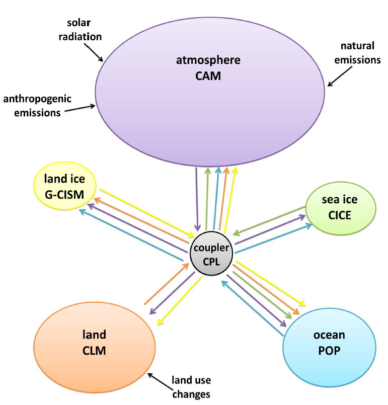
Enlarge  Diagram of software architecture for the Community Earth System Model. Coupled models use interacting components simulating different parts of the climate system. Bubble size represents the number of lines of code in each component of this particular model. Kaitlin Alexander, Steve Easterbrook

In order to gain useful insights, we need climate models that behave realistically. Climate modelers are always working to develop an ever more faithful representation of the planet’s climate system. At every step along the way, the models are compared to as much real-world data as possible. They’re never perfect, but these comparisons give us a sense for what the model can do well and where it veers off track. That knowledge guides the use of the model, in that it tells us which results are robust and which are too uncertain to be relied upon.

Andrew Weaver, a researcher at the University of Victoria, uses climate models to study many aspects of the climate system and anthropogenic climate change. Weaver described the model evaluation process as including three general phases. First, you see how the model simulates a stable climate with characteristics like the modern day. “You basically take a very long run, a so-called ‘control run,'” Weaver told Ars. “You just do perpetual present-day type conditions. And you look at the statistics of the system and say, 'Does this model give me a good representation of El Niño? Does it give me a good representation of Arctic Oscillation? Do I see seasonal cycles in here? Do trees grow where they should grow? Is the carbon cycle balanced?' ”

Next, the model is run in changing conditions, simulating the last couple centuries using our best estimates of the climate “forcings” (or drivers of change) at work over that time period. Those forcings include solar activity, volcanic eruptions, changing greenhouse gas concentrations, and human modifications of the landscape. “What has happened, of course, is that people have cut down trees and created pasture, so you actually have to artificially come in and cut down trees and turn it into pasture, and you have to account for this human effect on the climate system,” Weaver said.

The results are compared to observations of things like changing global temperatures, local temperatures, and precipitation patterns. Did the model capture the big picture? How about the fine details? Which fine details did it simulate poorly—and why might that be?

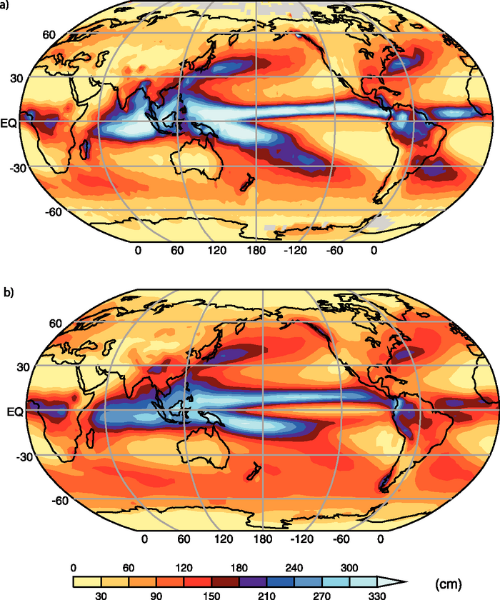
Enlarge Comparison of observed (top) and simulated (bottom) average annual precipitation 

between 1980 and 1999.IPCC

At this point, the model is set loose on interesting climatic periods in the past. Here, the observations are fuzzier. Proxy records of climate, like those derived from ice cores and ocean sediment cores, track the big-picture changes well but can’t provide the same level of local detail we have for the past century. Still, you can see if the model captures the unique characteristics of that period and whatever regional patterns we’ve been able to identify.

This is what models go through before researchers start using them to investigate questions or provide estimates for summary reports like those produced for the Intergovernmental Panel on Climate Change (IPCC).

Coding the climate

Some voices in the public debate over climate science have been critical of the fact that there is no standardized, independent testing protocol for climate models like those used for commercial and engineering applications. Climate scientists have responded that climate models are so different as to make such an “independent verification and validation” process incompatible.

Steve Easterbrook, a professor of computer science at the University of Toronto, has been studying climate models for several years. “I'd done a lot of research in the past studying the development of commercial and open source software systems, including four years with NASA studying the verification and validation processes used on their spacecraft flight control software,” he told Ars.

When Easterbrook started looking into the processes followed by climate modeling groups, he was surprised by what he found. 

“I expected to see a messy process, dominated by quick fixes and muddling through, as that's the typical practice in much small-scale scientific software. What I found instead was a community that takes very seriously the importance of rigorous testing, and which is already using most of the tools a modern software development company would use (version control, automated testing, bug tracking systems, a planned release cycle, etc.).”

“I was blown away by the testing process that every proposed change to the model has to go through,” Easterbrook wrote. 

“Basically, each change is set up like a scientific experiment, with a hypothesis describing the expected improvement in the simulation results. The old and new versions of the code are then treated as the two experimental conditions. They are run on the same simulations, and the results are compared in detail to see if the hypothesis was correct. Only after convincing each other that the change really does offer an improvement is it accepted into the model baseline.”

Easterbrook spent two months at the UK Met Office Hadley Centre, observing and describing the operations of the climate modeling group (which is about 200 scientists strong). He looked at everything from code efficiency to debugging to the development process. He couldn’t find much to critique, concluding that “it is hard to identify potential for radical improvements in the efficiency of what is a ‘grand challenge’ science and software engineering problem.”

Easterbrook has argued against the idea that an independent verification and validation protocol could usefully be applied to climate models. One problem he sees is that climate models are living scientific tools that are constantly evolving rather than pieces of software built to achieve a certain goal. There is, for the most part, no final product to ship out the door. There's no absolute standard to compare it against either.

To give one example, adding more realistic physics or chemistry to some component of a model sometimes makes simulations fit some observations less well. Whether you add it or not then depends on what you're trying to achieve. Is the primary test of the model to match certain observations or to provide the most realistic possible representation of the processes that drive the climate system? And which observations are the most important to match? Patterns of cloud cover? Sea surface temperature?

As more features have been added, current models have become much more sophisticated than models were 20 years ago, so the standards by which they're judged have tightened. It's entirely possible that earlier models would have failed testing that today’s models would pass. But that doesn't mean that the older models were useless; they may have just gotten fewer physical processes right or had a much lower resolution.

If, as Easterbrook argues, the models are essentially manifestations of the scientific community’s best available knowledge, there’s already a process in place to evaluate them—science. Experiments are replicated by other groups using their own models. Individual peer-reviewed studies are considered in the context of the accumulated knowledge of climate science. Climate models are not so different from other methods of inquiry in that a new scientific method must be invented especially for them.

Firing up the wayback machine

The individual researchers who are part of these modeling efforts work on very different aspects of the model, and each requires a slightly different way of doing things. Bette Otto-Bliesner works on the Community Earth System Model at the National Center for Atmospheric Research (which recently opened a new supercomputing center). Her research focuses on using climate models to understand past climate, working out the mechanisms that drove the events recorded in things like ocean sediment cores. “My research goal is to understand the uncertainties in the climate and Earth system responses to forcings using past time periods to provide more confidence in our projections of future change,” Otto-Bliesner told Ars.

Proxy records of climate from cores of ice or ocean sediments are limited to providing information about the geographic area from which they were collected, so climate models can help fill in the rest of the global picture. A model simulation of actual events—say, an immense ice-dammed lake draining into the North Atlantic and disrupting ocean circulation—can be compared to a network of proxy records to see if the simulated climate impact is consistent with what the proxies show. If the match is poor, then perhaps the observed change in climate was caused by something else.

Otto-Bliesner’s group is working to take this comparison one step further by having the model simulate the processes that create the proxy records as well. Instead of comparing the model to the interpretation of the proxy record data (such as temperature changes inferred from shifting isotope ratios), that data could be compared directly to a virtual version of the isotopes themselves, one produced by the model.

These paleoclimate simulations can serve to evaluate a model as well. The model can be run for interesting time periods, like the end of the last ice age, to see how well it simulates changes in temperature and ocean circulation. “We want to keep our paleo-simulations [separate] as an independent test of our models to changed forcings, so they are not included in the development process,” Otto-Bliesner told Ars. Since the climate was very different at times in the past, these tests help illuminate a model’s strengths and weaknesses.

Enlarge / Snapshot from an experiment simulating the last 22,000 years. In the graph at the bottom, 

the dark line represents simulated surface temperature over Greenland and the lighter line shows 

data from a Greenland ice core. National Center for Atmospheric Research/ University Corporation for Atmospheric Research

Setting the bar

Gavin Schmidt, a climate researcher at the NASA Goddard Institute for Space Studies, is more involved in the development itself. “I explore issues like how one evaluates [climate] models, how comparisons between models and observations should be done, and how one builds credibility in predictions,” he told Ars.

Improving the model means better simulating physical processes, Schmidt says, which doesn’t necessarily improve the large-scale match with every set of observations. “There are always observational datasets that show a mismatch to the model—either regionally or in time,” Schmidt explained. “Some of these mismatches are persistent (i.e., we haven't found any way to alleviate them); some are related to issues/parameters that we have more of a handle on, and so they can be reduced in the next iteration. One problem is that in fixing one problem one often makes something else worse. Therefore, it is a balancing act that each model center does a little differently.”

One surprisingly common misconception about climate models is that they’re just exercises in curve-fitting. The global average temperature record is fed into the model, which matches that trend and spits out a simulation just like it. In this (mistaken) view, having a model that compares well with reality is a necessary outcome of the process. This doesn’t demonstrate that climate models can be trusted to usefully project future trends, but this line of thinking is mistaken for several reasons.

There’s obviously more to a climate model than a graph of global average temperature. Some parameterizations—those stand-ins for processes that occur at scales finer than a grid cell—are tuned to match observations. After all, they are attempts to describe a process in terms of its large-scale results. But successful parameterizations aren’t used as a gauge of how well the model is reproducing reality. “Obviously, since these factors are tuned for, they don't count as a model success. However, the model evaluations span a much wider and deeper set of observations, and when you do historical or paleoclimate simulations, none of the data you are interested in has been tuned for,” Schmidt told Ars.

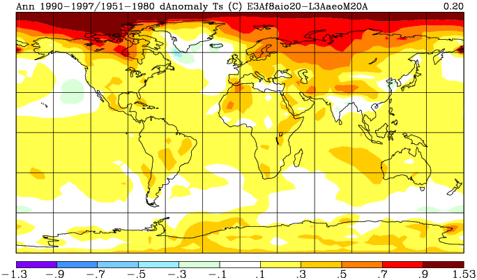
Enlarge / Example output showing average annual surface temperature from the NASA GISS ModelE.

NASA GISS

Why so cirrus?

Many of the most important parameterizations involve the complex behavior of clouds. Representing these processes effectively in a climate model is a key challenge, not just because they happen at scales far smaller than grid cells but because clouds play such a big role in the climate system. Storm patterns affect regional climate in many ways, and the way clouds respond to a warming climate could either enhance or partially offset the temperature change.

Tony Del Genio, another researcher at the NASA Goddard Institute for Space Studies, works on improving the way models simulate clouds. “The real world is more complicated than any model of it,” Del Genio told Ars. “Given the limited computing and human resources, we have to prioritize. We try to anticipate which processes that are missing from the model might be most important to include in the next-generation version (not everything that happens in the atmosphere is important to climate).”

“Once we identify a physical process we want to add or improve, we start with whatever fundamental understanding of the process that we have, and then we try to develop a way to approximately represent it in terms of the variables in the model (temperature, humidity, etc.) and write computer code to represent that,” Del Genio said. “We then run the model with the new process in it and we look for two things: whether the process as we have portrayed it behaves the way it does in the real world and whether or not it makes some aspect of the model's climate more realistic. We do this by comparison to observations, either field experiment, satellite, or surface remote sensing observations, or by comparing to fine-scale models that simulate individual cloud systems.”

Del Genio says that while modelers used to focus more on whether the model simulations looked like the average conditions for an area, they’ve learned that other types of behavior—like large-scale weather patterns— are better indicators of the usefulness of a model for projecting into the future. “A good example of that is something called the Madden-Julian Oscillation (MJO for short), which most people in the US have probably never heard of,” Del Genio said. “The MJO causes alternating periods of very rainy and then mostly clear weather over periods of a month or so over the Indian Ocean and in southeast Asia and is very important to people in that part of the world. It also affects winter rainfall in the western US. It turns out that whether a model simulates the MJO or not depends strongly on how one represents the clouds that develop into thunderstorms in the model, so we observe it closely and try hard to get it right.”

Del Genio also gets to apply his knowledge and skills to other planets. Using the extremely limited information we have about the atmospheres of other planets, models can help work out how they behave. “For other planets, we are still asking basic questions about how a given planet's atmosphere works—how fast do its winds blow and why, does it have storms like those on Earth, are those storms made of water clouds like on Earth, and why one planet differs from another,” Del Genio said.

Ice, on the rocks

While Tony Del Genio has his head in the clouds and outward into the Solar System beyond, Penn State glaciologist Richard Alley stands on ice sheets miles thick, thinking about what’s going on beneath his feet. Instead of trying to model the whole climate system, he’s focused on the behavior of valley glaciers and ice sheets. “An ice sheet is a two-mile-thick, one-continent-wide pile of old snow squeezed to ice under the weight of more snow and spreading under its own weight,” Alley told Ars. “The impetus for flow is essentially the excess pressure inside the ice compared to outside, and it's usually quantified as being the product of the ice density, gravitational acceleration, thickness of ice above the point you're talking about, and surface slope.”

Ice sheet models use the equations that describe that flow of ice to simulate how the ice sheet changes over time in response to outside factors. The size of an ice sheet, like a bank account, is determined by the balance of gains and losses. Increase the amount of melting going on at the edges of the ice sheet and it will shrink. Increase the amount of snowfall over the cold, central region of the ice sheet and it will grow. Lubricate the base of the ice sheet with liquid water, and it may flow faster to the sea, causing an overall loss of ice.

These models are complex and detailed enough that they’re usually run on their own rather than within a climate model that is already busy trying to handle the rest of the planet. Depending on the experiment being run with the model, climate conditions simulated by another model might be imported or a simpler, pre-determined scenario might suffice.

Like global climate models, ice sheet models can also be evaluated against what we know about the past. “Does the model put ice in places that ice was known to have been and not in places where ice was absent?” Alley said. “Are the fluctuations of ice in response to orbital forcing in the past configuration consistent with the reconstructed changes in sea level based on coastal indicators or isotopic composition of the ocean as inferred from ratios in particular shells in sediment cores?”

All this work eventually contributes to our understanding of how the ice sheet is likely to behave in the future. “For these projections to be reliable, we want to see similar behavior in a range of models, from simple to complex, run by different groups, and to understand physically why the models are producing the results they do; we're especially confident if the paleoclimatic record shows a similar response to similar forcings in the past, and if we see the projected behavior emerging now in response to the recent human and natural forcings,” Alley said. “With all four—physical understanding, agreement in a range of models, observed in paleo and emerging now—we're pretty confident; with fewer, less so.”

Along with providing better estimates of how ice sheets will contribute to sea level rise, ice sheet models also help generate research questions. By revealing the biggest sources of uncertainty, models can point to the types of measurements and research that will yield the greatest bang for the buck.

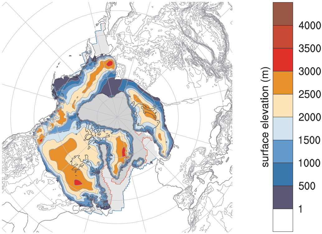
Enlarge  Simulation of ice sheet elevation at the peak of the last ice age using the Parallel Ice 

Sheet Model and the ECHAM5 climate model. Florian Ziemen, Christian Rodehacke, 

Uwe Mikolajewicz (Max Planck Institute for Meteorology)

Community service

There’s another way in which these climate models are probed—by comparing them with each other. Since there are so many groups of researchers independently building their own models to approximate the climate system, the similarities and differences of their simulations can be illuminating.

Observational data is necessarily limited, but every single thing in a model can be examined. That makes model-to-model comparison more of an apples-to-apples affair when they’re run using the same inputs (like greenhouse gas emissions scenarios). The cause of a poor match between some portion of a model and reality isn’t always obvious, whereas it could jump out when the results are compared to those produced by another model.

There are many such “model intercomparison projects,” including ones focused on atmospheric models, paleoclimate simulations, or geoengineering research. The largest is the Coupled Model Intercomparison Project (CMIP), which has become an important resource for the Intergovernmental Panel on Climate Change reports. What started in 1995 as a simple project blossomed into an enormously useful organizing force for an abundance of research.

Each phase of the project includes a set of experiments chosen by the modeling community. In the latest round, for example, the models have been investigating short-term, decadal predictions, the way clouds change in a warming climate, and a new technique for making comparisons between model results and atmospheric data from satellites.

Apart from helping research groups improve their models, CMIP also makes climate simulations from all the models involved accessible to other researchers. Interested in the future behavior of Himalayan glaciers? Or the economic impact of changes in precipitation over the US? Simulations from a variety of models for a range of emissions scenarios are conveniently available in one place and in standardized formats. In a way, that coordination also increases the value of the studies that use this data. If three different studies on species migration caused by climate change each used arbitrarily different scenarios for the future, comparing their results could be more difficult.

The most visible product of CMIP has probably been its contribution to the IPCC reports. When the reports show model ensembles (many simulations averaged together), they’re pulling from the CMIP collection. Rather than choosing a preferred model, the IPCC essentially works from the average of all of them, while the range of their results is used as an indicator of uncertainty. In this way, the work of independent modeling groups around the world is aggregated to help inform policy makers.

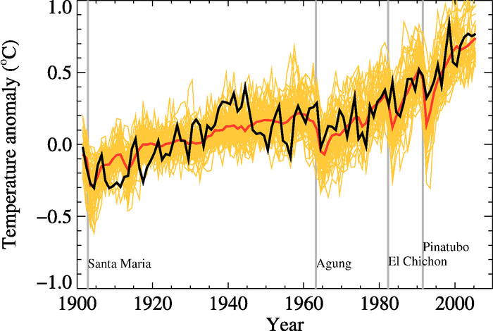
Enlarge  Average (red line) of 58 model simulations (yellow lines) of global average temperature 

compared to observations (black line).IPCC

No crystal ball—but no magic 8 ball, either

If you only tune in to public arguments about climate change or read about the latest study that uses climate models, it’s easy to lose sight of the truly extraordinary achievement those models represent. As Andrew Weaver told Ars, “What is so remarkable about these climate models is that it really shows how much we know about the physics and chemistry of the atmosphere, because they’re ultimately driven by one thing—that is, the Sun. So you start with these equations, and you start these equations with a world that has no moisture in the atmosphere that just has seeds on land but has no trees anywhere, that has an ocean that has a constant temperature and a constant amount of salt in it, and it has no sea ice, and all you do is turn it on. [Flick on] the Sun, and you see this model predict a system that looks so much like the real world. It predicts storm tracks where they should be, it predicts ocean circulation where it should be, it grows trees where it should, it grows a carbon cycle—it really is remarkable.”

But climate scientists know models are just scientific tools—nothing more. In studying the practices of climate modeling groups, Steve Easterbrook saw this firsthand. “One of the most common uses of the models is to look for surprises—places where the model does something unexpected, primarily as a way of probing the boundaries of what we know and what we can simulate," he said. "The models are perfectly suited for this. They get the basic physical processes right but often throw up surprises in the complex interactions between different parts of the Earth system. It is in these areas where the scientific knowledge is weakest. So the models help guide the scientific process."

“So I have tremendous respect for what the models are able to do (actually, I'd say it's mind-blowing), but that's a long way from saying that any one model can give accurate forecasts of climate change in the future on any timescale," Easterbrook continued. “I'm particularly impressed by how much this problem is actively acknowledged and discussed in the climate modeling community and how cautious the modelers are in working to avoid any possible over-interpretation of model results.”

“One of the biggest sources of confidence in the models is that they give results that are broadly consistent with one another (despite some very different scientific choices in different models), and they give results that are consistent with the available data and current theory,” Easterbrook said. And while they're being developed, the rest of the broad field of climate science is hard at work gathering more data and developing our theoretical understanding of the climate system—information that will inform the next generation of models.

The guiding principle in modeling of any kind was summarized by George E.P. Box when he wrote that “all models are wrong, but some are useful.” Climate scientists work hard to ensure that their models are useful, whether to understand what happened in the past or what could happen in the future.

Every projection showing multiple scenarios for future greenhouse gas emissions illustrates the present moment as a constantly shifting crossroads—the point where all future paths diverge, with their course determined using climate models. Armed with that map, we get to decide which of the possible paths we are going to make reality. The more we understand about the climate system and the more realistically climate models behave, the more detailed that map becomes. There’s always more to work out, but we’ve already advanced well past the stage where we need to ask for directions.

http://arstechnica.com/science/2013/09/why-trust-climate-models-its-a-matter-of-simple-science/