Death Spiral Watch: Experts Warn ‘Near Ice-Free Arctic In Summer’ In A Decade If Volume Trends Continue

by Joe Romm, Climate Progress, September 5, 2012

The sharp drop in Arctic sea ice area has been matched by a harder-to-see — but equally sharp — drop in sea ice thickness. The combined result has been a collapse in total sea ice volume.

Many experts now say that if recent volume trends continue we will see virtually ice-free conditions sometime in the next ten years. And that may well usher in a permanent change toward extreme, prolonged weather events “Such As Drought, Flooding, Cold Spells And Heat Waves.”

It will also accelerate global warming in the region, which in turn will likely accelerate both the disintegration of the Greenland ice sheet and the release of the vast amounts of carbon currently locked in the permafrost.

The European Space Agency’s CryoSat-2 probe confirms what the Pan-Arctic Ice Ocean Modeling and Assimilation System (PIOMAS) at the Polar Science Center has been saying for years: Arctic sea ice volume has been collapsing faster than sea ice area (or extent) because the ice has been getting thinner and thinner.

In fact, the latest satellite CryoSat-2 data shows the rate of loss of Arctic sea ice is “50% higher than most scenarios outlined by polar scientists and suggests that global warming, triggered by rising greenhouse gas emissions, is beginning to have a major impact on the region,” as the UK Guardian reported last month:

If the current annual loss of around 900 cubic kilometres continues, summer ice coverage could disappear in about a decade in the Arctic.

I have focused on sea ice volume for the past 6 years, since I was fortunate enough to hear Dr. Wieslaw Maslowski of the Oceanography Department at the Naval Postgraduate School in a 2006 American Meteorological Society seminar.  He reported that models suggested Arctic ice volume had dropped sharply since the mid 1990s. He then made an alarming forecast:

“If this trend persists for another 10 years–and it has through 2005–we could be ice free in the summer.”

That was in 2006, so he was talking about the possibility of being ice free in 2016.

Looking at volume and thickness helped me avoid the mistake that so many others made in thinking that the sea ice “recovered” after the 2007 minimum in sea ice extent.  The scientific literature and actual observations continued to vindicate Maslowski’s projection.

Since Maslowski’s warning appears to now have been vindicated by the CryoSat-2 data, I asked him for a comment. He said he didn’t want to comment on that data specifically until he’s seen the published results — since there are many inherent uncertainties involved. But he then added:

Regardless of all these uncertainties and for the record, if any of these estimates of arctic sea ice volume decline is close to reality, a near ice-free Arctic in summer can happen not in 2100, 2050 or 2037 but much sooner. One of the main reasons I believe it will happen sooner (i.e. the trend of sea ice volume decline will continue) is that with the shrinking sea ice cover in summer the Arctic Ocean increases its net annual heat content through absorption and redistribution, especially in the upper water column, below the surface mixed layer.

This constitutes a positive feedback to sea ice melt in addition to ice-albedo and other feedbacks, mainly because it can affect the sea ice cover year around, including in winter through upward heat entrainment and reduction of ice growth. The warmer Arctic Ocean can also affect air temperatures and circulation, not only during freeze-up but also in winter and spring. Observational evidence (Jackson et al., 2010 and 2011) suggests increasing sub-surface temperatures and over increasing area in the Canada Basin through 2009, which independently of models supports the argument about the increasing upper ocean heat content.

I do realize that the above sounds ‘alarmist’ and I’ve heard such criticism more than once before but I believe it’s my obligation to make sure that this message is heard by the policymakers and general public.

Maslowski did not make a new timing prediction, but instead directed me to a recent article he was lead author on, “The Future of Arctic Sea Ice,” in Annual Review of Earth and Planetary Sciences.

That article estimated a loss of 1,120 cubic kilometres per year from 1996 to 2007, quite close to the recently reported CryoSat-2 measurements. It continued:

Given the estimated trend and the volume estimate for October–November of 2007 at less than 9,000 km³ (Kwok et al. 2009), one can project that at this rate it would take only 9 more years or until 2016 ± 3 years to reach a nearly ice-free Arctic Ocean in summer. Regardless of high uncertainty associated with such an estimate, it does provide a lower bound of the time range for projections of seasonal sea ice cover.

This is the same estimate Maslowski made in 2006, although he has couched it more conservatively here and has explained that he wouldn’t be surprised if some summer ice lingers above Greenland and Eastern Canada into the 2020s. That’s why he uses the term “nearly ice-free.”

What’s interesting is that the volume trend has in fact continued according to PIOMAS and CryoSat-2. Many other experts are warning that we have effectively passed the point of no return and nearly ice-free are imminent. Fen Montaigne, senior editor of Yale e360, reports:

Peter Wadhams, who heads the Polar Ocean Physics Group at the University of Cambridge and who has been measuring Arctic Ocean ice thickness from British Navy submarines, says that earlier calculations about Arctic sea ice loss have grossly underestimated how rapidly the ice is disappearing. He believes that the Arctic is likely to become ice-free before 2020 and possibly as early as 2015 or 2016 — decades ahead of projections made just a few years ago.

Mark Drinkwater, mission scientist for the European Space Agency’s CryoSat satellite and the agency’s senior advisor on polar regions, said he and his colleagues have been taken aback by the swiftness of Arctic sea ice retreat in the last 5 years. “If this rate of melting [in 2012] is sustained in 2013, we are staring down the barrel and looking at a summer Arctic which is potentially free of sea ice within this decade,” Drinkwater said in an e-mail interview.

Wadhams told the BBC how much warming is accelerated by just replacing the reflective white ice with the more absorptive open ocean:

Prof Wadhams calculates that this increased absorption of the sun’s rays is “the equivalent of about 20 years of additional CO2 being added by man”.

The Cambridge University expert says that the Arctic ice cap is “heading for oblivion.”

Not every expert thinks the Arctic will be necessarily be nearly ice free by 2020. And Dr Seymour Laxon who has been working on the CryoSat-2 data said this of the 2020 projection:

Laxon urged caution, saying: “First, this is based on preliminary studies of CryoSat figures, so we should take care before rushing to conclusions. In addition, the current rate of ice volume decline could change.” Nevertheless, experts say computer models indicate rates of ice volume decline are only likely to increase over the next decade.

But whenever the nearly ice free conditions occur (and I’ve long been in the camp that says it’ll be by 2020), those who think we have not effectively crossed a point of no return — those who think we are not in a death spiral — are not paying attention to the thickness and volume analysis. As Yale e360 reported:

Jay Zwally, chief cryospheric scientist at NASA’s Goddard Space Flight Center and an observer of Arctic ice for 40 years, places little stock in the likelihood of a reversal of disappearing Arctic ice. New satellite technology has given scientists the ability to measure the height of sea ice above the water, and hence ice volume. Those measurements, he said, have vividly underscored that Arctic sea ice is in a swoon.

For example, a recent analysis of data from CryoSat and NASA’s ICESat satellite estimates that the volume of sea ice in a large area of the central Arctic Ocean has plummeted in late winter — February and March — by nearly half in just eight years, from an estimated 13,000 cubic kilometers in 2004 to 7,000 cubic kilometers in 2012.

“We’ve gone through a tipping point, and of all the things a tipping point applies to, sea ice is the most appropriate, because the idea is when it goes below a certain thickness it doesn’t go back under present conditions,” said Zwally. “People can get hung up on the specifics and lose track of the big picture, which is that it’s getting worse and it’s going to get [even] worse.”

And that has serious consequences for every person on this planet and countless future generations.

http://thinkprogress.org/climate/2012/09/05/799761/death-spiral-watch-experts-warn-near-ice-free-arctic-in-summer-in-a-decade-volume-trends-continue/

Fen Montaigne: Arctic Tipping Point: A North Pole Without Ice

Arctic Tipping Point:
A North Pole Without Ice

Scientists say this year’s record declines in Arctic sea ice extent and volume are powerful evidence that the giant cap of ice at the top of the planet is on a trajectory to largely disappear in summer within a decade or two, with profound global consequences.

by fen montaigne, yale360, August 30, 2012

As the northern summer draws to a close, two milestones have been reached in the Arctic Ocean — record-low sea ice extent, and an even more dramatic new low in Arctic sea ice volume. This extreme melting offers dramatic evidence, many scientists say, that the region’s sea ice has passed a tipping point and that sometime in the next decade or two the North Pole will be largely ice-free in summer.

NASA and U.S. ice experts announced earlier this week that the extent of Arctic sea ice has dropped to 4.1 million square kilometers (1.58 million square miles) — breaking the previous record set in 2007 — and will likely continue to fall even farther until mid-September. As the summer melt season ends, the Arctic Ocean will be covered with 45 percent less ice than the average from 1979 to 2000.

Click to enlarge

NASA

On August 26, 2012, Arctic sea ice reached a new record-low summer extent.

Even more striking is the precipitous decline in the volume of ice in the Arctic Ocean. An analysis conducted by the University of Washington’s Pan Arctic Ice Ocean Model Assimilation System (PIOMAS) estimates that sea ice volumes fell in late August to roughly 3,500 cubic kilometers — a 72-percent drop from the 1979-2010 mean.

Peter Wadhams, who heads the Polar Ocean Physics Group at the University of Cambridge and who has been measuring Arctic Ocean ice thickness from British Navy submarines, says that earlier calculations about Arctic sea ice loss have grossly underestimated how rapidly the ice is disappearing. He believes that the Arctic is likely to become ice-free before 2020 and possibly as early as 2015 or 2016 — decades ahead of projections made just a few years ago.

Mark Drinkwater, mission scientist for the European Space Agency’s CryoSat satellite and the agency’s senior advisor on polar regions, said he and his colleagues have been taken aback by the swiftness of Arctic sea ice retreat in the last 5 years. “If this rate of melting [in 2012] is sustained in 2013, we are staring down the barrel and looking at a summer Arctic which is potentially free of sea ice within this decade,” Drinkwater said in an e-mail interview.

A small number of climate scientists say that natural variability may be playing a significant role in the rapid retreat of Arctic sea ice, intensifying human-caused climate change, and they caution against predicting the imminent demise of the region’s summer sea ice. But an 

Extraordinarily low ice levels indicate the summer sea ice has passed a point of no return.

overwhelming majority of Arctic ice experts say that recent data offer powerful evidence that summer sea ice has passed a point of no return.

The dramatic ice loss is being driven by a several key factors, scientists say. Chief among them is that decades of warming have so extensively melted and thinned Arctic sea ice that rapidly expanding areas of dark, open water are absorbing ever-greater amounts of the sun’s radiation, further warming the region in a vicious cycle.

Second, swiftly warming air and ocean temperatures in the Arctic have, for now at least, altered atmospheric activity, with two consequences: Warmer air is being pulled into the Arctic, and increased storms and cyclones in summer are not only driving ice out of the Arctic basin, but also breaking up the ice pack and further exposing more dark water.

And finally there is the inescapable reality that steadily rising levels of carbon dioxide being pumped into the atmosphere by human activity are continuing to warm the Arctic and the rest of the globe, further hastening the loss of Arctic Ocean ice. Several experts say that the only thing that could slow this disappearance — and then only for a few years — would be a major volcanic eruption that reduces the amount of the sun’s energy striking the earth.

“It’s sobering to see the Arctic change so rapidly,” said Ted Scambos, senior research scientist at the National Snow & Ice Data Center in Colorado. “Simply staring at the satellite data that we’re seeing every day is awesome, but in a sad sort of way. It doesn’t look like the Arctic anymore. The summer ice used to look like a cap that nearly filled the Arctic basin. It now looks like a raft with room on every side. You can imagine what it’s going to 

‘The summer ice used to look like a cap…. It now looks like a raft with room on every side.’

look like when the North Pole is open water, when there is only a tiny amount of ice left in August and September. The planet will look a lot different.”

The loss of the great white dome of ice at the top of the world in summer will have profound effects, scientists say. These include a reduction of the amount of solar radiation reflected back into space by the ice, significant changes to the jet stream and Northern Hemispheric weather patterns, and even-more rapid warming in the far north, speeding the melting of Greenland’s massive ice sheets and increasing global sea levels.

In addition to these impacts, said Drinkwater, “Increased storminess will generate ocean wave systems which, un-damped by the presence of sea ice, will pound the circumpolar north coastlines. Current rates of coastal permafrost degradation will be accelerated, leading to significant coastal erosion and reconfiguration of the high-latitude shoreline. Meanwhile, we have also recently heard about the potential for release of sub-sea methane deposits and thereby an acceleration of the current greenhouse effect.”

The record low sea ice extent in 2007 of 4.2 million square kilometers was due to some unusual circumstances, including a sunny summer in the Arctic and higher temperatures. Summer sea ice extent rebounded somewhat in the next several years, rising to 5.3 million square kilometers in 2009, giving some hope to mainstream scientists that Arctic sea ice was not in a “death spiral.”

But Scambos and other experts say that recent data on plummeting ice extent and volume show that the Arctic has entered a “new normal” in which ice decline seems irreversible. Because of thinning ice and swiftly expanding areas of open water, the Arctic Ocean will no longer be kept frigid in summer by the reflectivity of snow and ice — the so-called ice-albedo effect, in which ice and snow reflect a high percentage of the sun’s energy back into space.

NASA

Melting Arctic sea ice.

Thick sea ice that formed over many years is increasingly rare in the Arctic. In the 1960s, submarines routinely encountered 12-foot-thick ice around the North Pole and 20-foot-thick ice in some other areas; now those regions often contain ice that is only three to four feet thick. Many parts of the Arctic Ocean are now covered with thin, year-old ice that melts quickly in spring and summer.

This spring, noted Scambos, extensive late winter snow cover on land melted unusually rapidly, reaching record low levels by June. Sea ice across much of the Arctic began to melt 10 to 14 days earlier than in the preceding few decades. Relatively clear skies from late May through June further hastened the melting of sea ice, but even as cloudier weather prevailed in July and August, the record sea ice retreat continued.

“The sensitivity of the Arctic to a warm summer is much higher now than it was in the 1990s or early 2000s,” said Scambos. “What we’re seeing last year and this year is that 2007 wasn’t a fluke. As we’ve gone forward a few years, we’re seeing that many different patterns of weather lead to significant sea ice loss in the Arctic.”

Scambos does not foresee summer sea ice in the Arctic largely disappearing this decade, estimating that such an event could occur around 2030, “plus or minus a decade.” He said the “endgame” of Arctic summer sea ice will probably mean that around 1 million square kilometers — about 15% of what existed in the mid-20th century — will remain in the Canadian High Arctic and some other regions, leaving the North Pole generally ice-free in August and September.

Drinkwater said that changing weather patterns, related to more heat and moisture being released into the Arctic atmosphere, have played a significant role in accelerating sea ice loss. Sea ice retreat in the past decade has been accompanied by a trend toward lower atmospheric pressure and more storms and cyclonic activity, which in turn breaks up

Changing weather patterns have played a significant role in accelerating sea ice loss.

the pack ice and exposes more open water. A powerful Arctic storm earlier this month did just that, Drinkwater noted.

He said that Arctic sea ice could conceivably rebound for some period of time if atmospheric circulation changes and a pattern known as the Arctic Oscillation — currently in a positive phase — moves into a negative phase and ushers in a period of prolonged high atmospheric pressure and fewer storms. This, said Drinkwater, would enable sea ice to remain trapped in the Arctic basin and thicken.

“However,” added Drinkwater, “this seems like blind hope in a system whose feedbacks all appear geared to getting rid of sea ice.”

Judith Curry [snip].

MORE FROM YALE e360

Linking Weird Weather to
Rapid Warming of the Arctic

The loss of Arctic summer sea ice and the rapid warming of the Far North are altering the jet stream over North America, Europe, and Russia. As Jennifer Francis writes, scientists are now just beginning to understand how these profound shifts may be increasing the likelihood of more persistent and extreme weather.
READ MORE

Jay Zwally, chief cryospheric scientist at NASA’s Goddard Space Flight Center and an observer of Arctic ice for 40 years, places little stock in the likelihood of a reversal of disappearing Arctic ice. New satellite technology has given scientists the ability to measure the height of sea ice above the water, and hence ice volume. Those measurements, he said, have vividly underscored that Arctic sea ice is in a swoon.

For example, a recent analysis of data from CryoSat and NASA’s ICESat satellite estimates that the volume of sea ice in a large area of the central Arctic Ocean has plummeted in late winter — February and March — by nearly half in just eight years, from an estimated 13,000 cubic kilometers in 2004 to 7,000 cubic kilometers in 2012.

“We’ve gone through a tipping point, and of all the things a tipping point applies to, sea ice is the most appropriate, because the idea is when it goes below a certain thickness it doesn’t go back under present conditions,” said Zwally. “People can get hung up on the specifics and lose track of the big picture, which is that it’s getting worse and it’s going to get [even] worse.”

http://e360.yale.edu/feature/tipping_point_arctic_heads_to_ice_free_summers/2567/

D. Bailey & M. Pelto: Zebras? In Greenland? Really? [Variations in Greenland Ice Sheet outlet glacier behavior]

Zebras? In Greenland? Really?

by Daniel Bailey and Mauri Pelto, Skeptical Science, April 11, 2012

At first glance, zebras are all the same.  Sure, you can argue that they are black with white stripes or white with black stripes.  But nobody really cares; they're zebras, after all.

[sorry, readers, in the interest of saving space the photo of the zebras is not posted -- but I am sure you will have no trouble imagining them]

Just as each zebra has an individualized set of stripes, making them unique, so also are each of the individual glaciers in Greenland unique.  They each have varied lengths, heights, widths, fjord geometries, differently-sized accumulation zones (where they "pack on weight") and flow speeds.  Each is located in a different part of Greenland and thus are also affected differently by their latitude, oceanic currents (for the marine-terminating glaciers), weather and climatic patterns.  And also by the modifying effects of Arctic amplification of the warming of the globe.

Variations in Greenland Ice Sheet outlet glacier behavior

The Greenland Ice Sheet has an area of 2.17 million square kilometers (1.28 million square miles) and spans 18 degrees of latitude from north to south.  It is not surprising that over this vast area that the geology and climate vary substantially and that this leads to variations in behavior of Greenland glaciers.  Our tendency is to lump the Greenland Ice Sheet into one category impacted similarly by each of the dynamic forces that impact flow. This is akin to saying banks, credit unions and savings and loan institutions are impacted similarly by all the economic forces.  In the case of a recession there is a shared signal, just as with global warming there is a shared signal amongst Greenland glaciers.   This is a simplification that does not work.  In this article we divide the glaciers into four main categories to illustrate the different properties and sensitiveness of each.

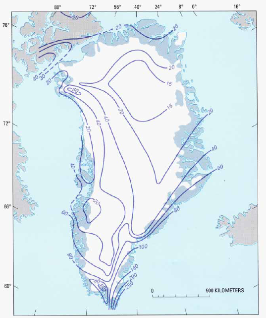
The surface mass balance of the glacier is the difference of accumulating snow on the ice sheet (its income) and snow and ice losses from melting and calving (its expenditures).  The volume of the ice sheet is its asset.  On an ice sheet, the main factor driving flow is simply the mass balance input in the accumulation zone.  The higher the accumulation rate the faster the movement; the accumulated snow is inexorably moved downslope towards the ocean and the margin of the ice sheet.  Observation of a precipitation map (focused not on the outer margin, but on the accumulation zone of the ice sheet) indicates that highest accumulation rates, over 40 cm per year, extend along the western side of the ice sheet to the southeast quadrant of the ice sheet.  

Figure 2. Distribution of precipitation in Greenland (in grams per square centimeter per year). Contours dashed where inferred. Ice-free areas are shown in dark gray. (USGS Satellite Image Atlas of Greenland)

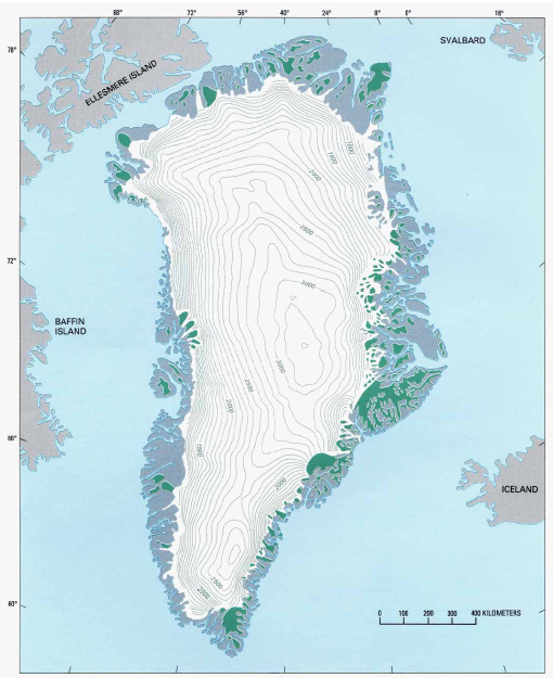
The overall topography of the ice sheet is controlled both by the basal and peripheral geology and the mass balance distribution of the ice sheet.  The higher rates of mass accumulation inland and the greater melting nearer the margin yield a steeper profile for the ice sheet. 

Figure 3. Topographic map of the Greenland ice sheet. The contour interval is 100 m. Local ice caps and ice domes are shown in green. Ice-free areas are shown in dark gray. (USGS Satellite Image Atlas of Greenland)

Figure 3 shows that the contours have the closest spacing along the west margin and in the southeast, just as the high accumulation rates in those areas would suggest.  Thus the combination of the surface slope and the accumulation rate drive faster flow in these regions. 

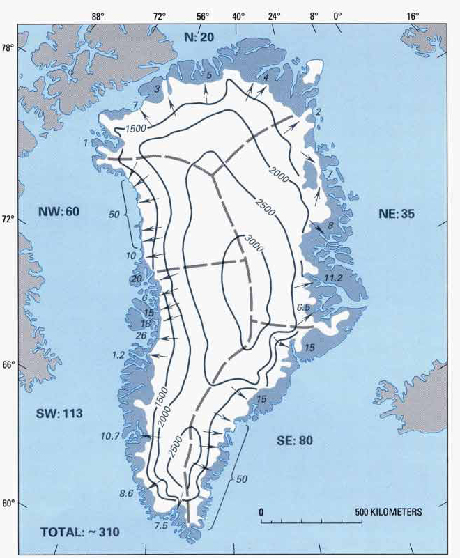
The generalized calving output of each section of the ice sheet (Figure 4, below) indicates the volume flux by quadrant and by glacier in some cases. 

Figure 4. Generalized calving output by quadrant, in cubic kilometers per year water equivalent based on the assumption of an equilibrium state. The contours indicate elevation in meters. (USGS Satellite Image Atlas of Greenland)

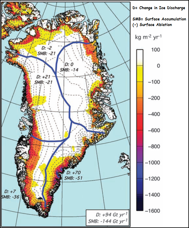
The northern quadrant is one of the largest in terms of the ice sheet perimeter, but the calving output is the lowest at 20 km³.  The northeast quadrant at 35 km³ is the second lowest.  The highest are the southwest and southeast quadrants at 113 and 80 km³, respectively.  The difference is the result of higher accumulation rates.   If we look at more recent work, which examines the changes in volume discharge and surface mass balance, we see the greatest discharge changes and surface loss are in the southeast. 

Figure 5. Higher calving flux indicates higher velocities (Van Den Broecke et al., 2009). D denotes change in ice discharge while SMB denotes the net surface mass balance (accumulation minus ablation).

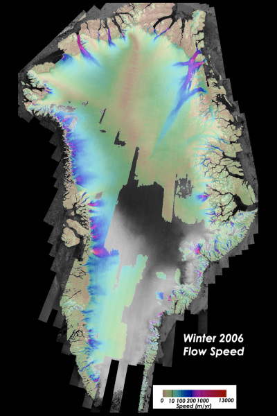
Figure 6. Ice flow speed in Greenland (color) for winter 2006 derived from synthetic aperture radar (SAR) imagery (gray scale image derived from NASA funded research). Because of the large range of speeds (1-13,000 m/yr), a log color scale is used (Ian Joughlin, Big Ice).

Hence the above velocity map of the glacier will indicate higher average velocities in the quadrants with the highest calving volume flux.  This map indicates relatively low flow rates of less than 10 m/year inland, with particular bands of fast flow that extend well into the ice sheet and feed outlet glaciers.  The variation in flow and accumulation rates indicates the problem of lumping the glaciers into one category. 

Climate change has led to an observed increase in surface melting, surface accumulation, increased discharge and overall mass balance losses.  The very mechanism that establishes the basics of behavior of the GIS mass balance are changing (Zwally et al., 2011).

Greenland glaciers fall into at least 4 common types, each with its own unique sensitivity to sea surface temperature, surface melting, meltwater lubrication, calving changes, etc.

Type 1: Northern, with Large Floating Termini

Northern glaciers with large floating termini (Petermann, Ryder, Steensby, Zachariae, Academy, etc).  Each of these is a marine terminating outlet glacier that has an extensive floating ice shelf.  The large ice shelves can exist in part due to the lower surface melt rates and the lower flow rates of the glacier.  Petermann Glacier is the fastest with a flow speed of 1,000 m/year at the grounding line.  This is much less than the average outlet glacier speed along the west coast.  The large floating ice shelves are susceptible to bottom melting but, except for Petermann Glacier, we have no observations of the process or that more warm water is penetrating under these ice shelves.  Rignot and Steffen (2008) found that at Petermann Glacier 80% of the ice loss into the ocean was from basal melting of the floating tongue.  If the ice shelves are removed, the feeding glacier is less buttressed and will accelerate for a period and draw down its surface profile.  The recent ice area lost by Petermann, Academy and Zachariae Ice Stream indicate these glaciers are being impacted by the increased melting at the surface and likely the base of the ice shelf for Petermann Glacier at least. 

Examination of how far the high velocities extend inland in Figure 6 indicates that it is only Zachariae and Petermann that tap far into the ice sheet.  This northern area has low accumulation rates, and a shorter less intense melt season.  The early onset of melting and lack of accumulation in 2010 led to an early exposure of the ablation zone on these glaciers. 

This is their sensitivity Achilles Heel:  relatively little increases in melt can expand the ablation zone appreciably given the low surface slopes and low accumulation rates.   Based on the velocity map, it is the Zachariae that is likely the only of this group that would be comparable to a bank that is too big to fail as its increased velocity band extends well into the ice sheet. 

Figure 7. Ice flow speed for Zachariae Glacier (Joughlin et al., 2010).

Type 2: Inland-terminating

Glaciers with inland termini lacking any calving (Sukkertoppen, Frederickshaab, Russell, etc.). Between the fast flowing marine terminating outlet glaciers, the ice sheet particularly in the southwest quadrant has numerous glaciers that terminate on land or in small lakes.  The velocity of these glaciers reaches a maximum of 1-2 meters/day.  Each terminates on land because total ablation over the glacier equals total accumulation at the terminus.  These glaciers are more like a typical alpine glacier and are susceptible to the forces that tend to cause alpine glaciers to experience peak flow during spring and early summer.  Those forces are the delivery of meltwater to the base of the glacier, when a basal conduit system is poorly developed.  This leads to high basal water pressure, which enhances sliding.  As the conduit system develops the basal water pressure declines as does sliding, even with more water.

Figure 8. Inland terminating glaciers (Sundal et al., 2011).

This is what has been recently reported to be the case by Sundal et al. (2011).  The meltwater lubrication mechanism is real, but as observed is limited both in time and area impacted.  It is likely that, as on alpine glaciers, the seasonal speedup is offset by a greater slowdown late in the melt season.  Most observed acceleration due to high meltwater input has been on the order of several weeks, leading to a 10-20% flow increase for that period.  The role of supraglacial lakes in this has been a point of emphasis; Luthje et al. (2006) noted that the area covered by supraglacial lakes was independent of the summer melt rate but controlled by topography.  This led Luthje et al. to conclude that  the area covered by supraglacial lakes will remain constant even in a warmer climate.  This suggests that the enhancement of flow by the drainage of such lakes would be limited.

The land terminating glaciers such as Sukkertoppen, Russell and Mittivakkat are retreating significantly in response to global warming.   This is an indication of negative mass balance. The latter glacier in southeast Greenland has retreated 1,200 meters since 1931 (Mernhild et al., 2011).  The Mernhild study identified this slow rate compared to the outlet glaciers and, based on mass balance observations, that the current surface mass balance can only support a glacier at most one-third its current size.   This indicates the slow but inexorable sensitivity of the non-calving glacier to surface mass balance change.  Moon and Joughin (2008) observed that the retreat of the land terminating glaciers was relatively minor from 1992 to 2007, averaging 5 m/year or less.  These glaciers are the equivalent in our banking system to the local banks:  there are many and they are sensitive, but the changes in a single one is not important. 

Type 3: Marine-terminating

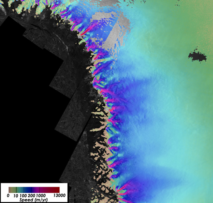
Fast flowing marine terminating outlet glaciers of western and southeast Greenland (Rinks, Umiamako, Helheim, Jakobshavn, Epiq Sermia, etc.).  These are the glaciers that drain the greatest area of the ice sheet and deliver the greatest volume to the oceans via calving.  The flux from many of the larger glaciers is over 10 km³/year (DMI).  Each of these glaciers is fast-flowing at the terminus; the fast flow section extends inland into the ice sheet up a sub-glacial trough.  The outlet glaciers act like a drain capturing ice from a larger area of the ice sheet than their narrow terminus would suggest.  

Figure 9. Marine-terminating glaciers (Thomas et al., 2009).

Pelto et al. (1989), in a paper on the equilibrium state of the Jakobshavn Glacier, showed that the terminus had not changed significantly in 30 years; its velocity had also been consistent.  Furthermore, it was observed that the velocity was consistent throughout the seasons.  This indicated that the glacier velocity was not being impacted by the meltwater pulse of summer. 

Bob Thomas (NASA, 2004) and Terry Hughes (University of Maine, 1986) developed the basic mechanism of flow for the glacier that has proven to be true.  The outlet glaciers have a balance of forces at the calving front.  The fjord walls, the fjord base and the water column impede flow.  The slope of the glacier, its upglacier velocity and the height of the calving face strive to increase flow.  If the glacier thins than there is less friction at the calving front from the fjord walls and the fjord base, leading to greater flow.  The enhanced flow leads to retreat and further thinning, resulting in the thinning and the acceleration spreading inland.  In 1990 it was not envisioned that acceleration would occur as soon as it has, yet that was the motivation for the research. 

Figure 10. Jakobshavn profile (Thomas et al., 2009).

In 2001, the acceleration of the Helheim, Jakobshavn and Kangerdlussaq Glaciers caught the attention of the world.  By 2007, acceleration had been noted at all 34 marine terminating outlet glaciers observed.

The acceleration was not significantly seasonal; Howat et al. (2010) noted a 15% seasonal component to the acceleration: it had spread inland and had led to retreat and thinning.  This demonstrated that the marine terminating glaciers were largely responding to a change in the balance of forces at the glacier front. 

Figure 11. Ice flow velocity as color over SAR amplitude imagery of Jakobshavn Isbræ in (a) February 1992 and (b) October 2000. In addition to color, speed is contoured with thin black lines at 1,000 m/yr intervals and with thin white lines at 200, 400, 600, and 800 m/yr. Note how the ice front has calved back several kilometers from 1992 to 2000. Further retreat in subsequent years caused the glaciers speed to increase to 12,600 m/yr near the front (Ian Joughlin, Big Ice).

The recent increases in outlet glacier discharge have always been coincident with floating tongue losses.   This causes reduced back pressure at the glacier front, letting up on the brakes; the resulting glacier thinning leads to less basal friction and further acceleration.  If the glacier front retreats into deeper water the process will continue and increase.  This is why understanding the basal slope changes inland of the calving fronts is crucial. Moon and Joughin (2008) observed the terminus change of 203 glaciers from 1992 to 2007 and noted a synchronous ice sheet wide retreat of tidewater outlet glaciers. The thinning could be due to increased surface melt, basal melt or most likely a combination of the two.  Moon and Joughin (2008) reported for the 2000-2006 period:

• In the southeast quadrant 35 glaciers retreated an average of 174 m/year
• In the eastern quadrant 21 glacier retreated an average of 106 m/year
• In the northwest 64 glaciers retreated an average of 118 m/year. 

Each quadrant’s retreat increased markedly after 2000.  The largest of this group are comparable to the banks that are too big for our banking system to allow them to fail:  they drain a substantial portion of the entire ice sheet and reach so far into the ice sheet that their behavior can impact that of other adjacent glaciers.

Type 4: Marine-terminating in Shallow Water

Marine terminating glaciers outlet glaciers in shallower water (Humboldt, Cornell, Steenstrup, etc.).  These glaciers do have calving termini but lack the large fast flowing feeder tongues extending into the glacier.  This is because there is not a topographic low under the ice sheet that funnels the flow.  Humboldt Glacier is the widest front of any Greenland glacier, wider even than Petermann Glacier. 

Figure 12. Humboldt profile (Thomas et al., 2009).

However, the velocity on average is low at 100 m/year, and the base of the glacier is quite high.  This makes it difficult for a large calving retreat of the glacier to occur and extend inland.  Humboldt Glacier is retreating but, as the velocity profile indicates, the glacier, despite its size, does not tap dynamically into the center of the ice sheet.  These glaciers are substantial, but their failure (though significant for sea level) would not destabilize the ice sheet as a whole.

 Greenland Ice Sheet outlet glaciers: Zebras no more

 Overall in Greenland, the rate of area loss in marine-terminating glaciers during the 2010 melt season (419 km²) was 3.4 times that of the previous 8 years. There is now clear evidence that the ice area loss rate of the past decade (averaging 120 km²/year) is greater than loss rates pre-2000.  The exceptional extension of the ablation season in 2010 in southern Greenland indicates the vulnerability of these areas to expanded melt regions (Box et al., 2010). 

The amazing aspect of Greenland glaciers is that (despite the specific variation in type, location specific fjord configuration, etc.) their response has been as uniform and synchronous to global warming as has been observed.  If this warming of the world persists long enough, the  ice “banks” of Greenland will begin to fail.  Those with the greatest reserves on their asset sheets and the fastest turnover, and thus having the greatest potential contributions to sea level rise over time, are:

• In the north, Zachariae (and to a lesser extent, Petermann)
• The fast flowing marine terminating outlet glaciers of western and southeast Greenland (Rinks, Umiamako, Helheim, Jakobshavn, Epiq Sermia and Kangerdlussaq)

---

Further Reading & Resources

1. Pelto et al. (1989)
2. Luthje et al. (2006)
3. Moon and Joughin (2008)
4. Rignot and Steffen (2008)
5. Thomas et al. (2009)
6. Van Den Broecke et al. (2009)
7. Box et al. (2010)
8. Howat et al. (2010)
9. Joughlin et al. (2010)
10. Mernhild et al. (2011)
11. Sundal et al. (2011)
12. Zwally et al. (2011)
13. The USGS Satellite Image Atlas of Greenland

http://www.skepticalscience.com/Variations_in_Greenland_Glaciers.html

The Zwally Effect: new evidence of its broader application to Greenland's ice sheet melting and glacier outflows

The Zwally effect: It won’t go away

by Graham Cogley, environmentalresearchweb.org, July 19, 2010

The Zwally effect is an acceleration of the flow of marginal ice in the ice sheets due to lubrication of the bed by meltwater percolating from the surface. Up to a point, this phenomenon is not surprising. It is well documented on smaller, thinner valley glaciers. The surprise, first documented by Zwally and co-authors in 2002, is seeing the same phenomenon in ice as thick as 1,200 m.

The Zwally paper has stimulated a growing literature with two main threads. One thread tries to explain how meltwater can find its way through more than a kilometre of ice. The other tends to show that the Zwally effect is not the reason for dramatic increases in the speed of tidewater outlet glaciers, where the evidence favours, quite strongly, warm ocean water as the culprit. But that doesn’t mean that seasonal acceleration is uninteresting.

Ian Bartholomew and co-authors report on more dramatic seasonal acceleration than has been measured hitherto. It still doesn’t rival the speed-ups observed on some tidewater outlets, but the observations highlight the potential of GPS from a different angle, and suggest fascinating insights into how the surface meltwater does its subglacial work.

This new report relies on time series of positions obtained with four Global Positioning System receivers deployed along 35 km of a land-terminating flowline at 67.1° N in southwest Greenland. The data include not just horizontal but also vertical velocities, as well as near-surface air temperature. Averaged over the summer, the speed-up from winter background values was rather modest. But the fascinating bits are the details.
The further up-glacier, the later the onset of speed-up, by more than a month. The natural explanation is a later onset of melting at higher elevations. The highest site was at 1,063 m and the lowest at only 390 m above sea level.

More interesting is that the horizontal velocity correlates very nicely with the vertical acceleration, or in other words with the rate of uplift of the surface. The ice goes faster when the surface is uplifting rapidly. Or rather, rapid uplift seems to provoke speed-up. This is a subtle observation in more ways than one. For one thing, the amounts of uplift are a few decimetres at most. That we can detect such subtle vertical motions is a payoff for all the trouble it took to loft a couple of dozen GPS satellites into orbit.

More interesting still is the authors’ subdivision of the summer into three phases. In phase 1, there is no particular surface uplift or speed-up: the meltwater, if any, has yet to reach the bed. In phase 2, the cumulative uplift increases towards a maximum, and so do the horizontal velocities, more or less. (You need the eye of faith to see these phases in the noisy data. But I buy them.) The concluding phase 3 sees repeated episodes of uplift and speed-up, but the course of the surface elevation is downward and so, more or less, is that of the horizontal velocity.

Phases 2 and 3 add up to another picture of an invisible world beneath the authors’ feet. The meltwater, once it reaches the bed, pressurizes the ice and forces it upwards, filling and enlarging cavities and promoting basal sliding. But the enlargement proceeds at least in part by melting of roofs and walls, implying the creation of connections and, in short, of a network. The network grows steadily better at discharging the arriving meltwater. Phase 2 becomes phase 3 when the network becomes more than able, on average, to cope with the spate of water. Phase 3 ends when the supply of meltwater gives out, and the ice starts winning again, resuming its regular wintertime job of squeezing the summertime channels shut.

If you want real glaciological drama, visual or acoustic, you should probably go to tidewater terminuses, at which most of the ice leaves the ice sheet. But there is still plenty of land-terminating ice, and the main things about the Zwally effect, granting that it is real, are that it must be real everywhere; and that if the surface of the ice sheet gets warmer, then the bed of the ice sheet is bound to get busier.

Link:  http://environmentalresearchweb.org/blog/2010/07/the-zwally-effect-it-wont-go-a.html