Blog Archive

Showing posts with label North Atlantic thermohaline circulation. Show all posts

Friday, December 16, 2016

Huge 20-Year Build up of Arctic Fresh Water May Flood North Atlantic & Stall Gulf Stream

by FishOutOfWater, DailyKos, December 13, 2016

http://www.whoi.edu/cms/images/Figure-3-for-BG-FWC-results_432873.jpg

"Figure 3 Time series of freshwater content in different layers of the Beaufort Gyre region. Blue bars depict total liquid freshwater content. Black bars show freshwater content in sea ice. Yellow bars – freshwater content in the mixed layer, red bars – in the Pacific and green bars – in the Atlantic water layer. Freshwater content is shown in thousand cubic kilometers. Upper left bars shows total annual freshwater flux into the Arctic Ocean from all rivers; green and black small bars show errors in liquid and sea ice freshwater content estimates. All freshwater contents are calculated relative to 34.8 reference water salinity." The build up in volume from 2002 to 2015 is about the volume of Lake Michigan which stores 4,918 cubic km of water.

Huge volumes of fresh water have been building up over the past 20 years in the Arctic waters north of Alaska. A volume the size of Lake Michigan built up from 2003 through the end of 2015. Before the 1990s, there were regular cycles of fresh water build up and release within decades as periods of high pressure north of Alaska were followed by periods of stormy weather. Scientists suspect that over the past 20 years large amounts of melt water from Greenland’s glaciers have changed the dynamics of the North Atlantic ocean and the Arctic atmosphere. Since the 1990s, a dome of high pressure has persisted in the Beaufort sea and the anticyclonic winds have pumped fresh water towards the high’s center building up a mound of relatively fresh water over a huge area north of Alaska. The primary source of the fresh water is rivers that flow into the Arctic. Over the past several decades, sea ice melting has added about 20%  to the increase of fresh water in the Beaufort sea.
The freshwater content of the Beaufort gyre  increased by a volume the size of lake Michigan from the 1970s to 2008.
The freshwater content of the Beaufort gyre  increased by a volume the size of lake Michigan from the 1970s to 2008.
A major 2008 report by a team of scientists led by Wood’s Hole oceanographer Andrey Proshutinsky found an increase of 5000 km3 of fresh water from the 1970s to 2008. www.whoi.edu/…
From 2008 to 2015 an additional 2000 km3 was added so the total increase in fresh water is 7,000km3. The total volume of the world’s second largest lake by volume, Lake Michigan, is just under 5,000km3.
Preliminary data from the BGOS 2008 cruise indicate that the FWCL in the BG continued to rise in 2008 and reached 21,000 km3– a historical maximum from all available years of observations. Compared to 1970s climatology (the pre-90s decade with the most extensive data coverage, (Figure 1) there has been a FWCL increase in the BG of approximately 5,000 km3. This is comparable with the volume of fresh water annually delivered to the Arctic Ocean by rivers and through Bering Strait (5700 km3 per year, Serreze et al., [2006]).
The freshwater layer in the Beaufort sea deepened by 3 meters - about 10 feet from 2003 to 2007. Because the Beaufort gyre covers a large area, this is a huge volume of fresh water. Persistent high pressure in 2007 caused Siberian and North American river water and water from a massive melt of sea ice to flow into this Arctic sea north of Alaska.
The freshwater layer in the Beaufort sea deepened by 3 meters - about 10 feet from 2003 to 2007. Because the Beaufort gyre covers a large area, this is a huge volume of fresh water. Anticyclonic winds associated with persistent high pressure in 2007 caused Siberian and North American river water and water from a record melt of sea ice in 2007 to flow into this Arctic sea north of Alaska.
The persistent anticyclonic Beaufort high pressure builds up a mound of water under it because the direction of a mass of water moves to the right of the wind  direction in the northern hemisphere because  the rotation of the earth gives the water spin. See this post at Neven’s sea ice blog by an Arctic oceanographer for details. neven1.typepad.com/...
On the other hand, cyclonic rotation associated with low pressure areas causes water to well up from below the center of the low. Thus  years of high pressure followed by  years of storminess cause moderate periodic surges of fresh water from the Arctic to the north Atlantic ocean. It was like the Arctic breathed in fresh water then breathed it out in a period of a decade or less. The largest observed freshwater surge called the “Great Salinity Anomaly” happened in the early 1970’s.
The Great Salinity anomaly was one of the likely causes of the brutal American winters of the 1970s. Fresh water tends to float over denser warm salty Gulf Stream water in sub-Arctic seas of the north Atlantic. This keeps the warm salty water from releasing its heat to the atmosphere and sinking thousands of feet into the deep Atlantic. This disruption of the thermohaline circulation is popularly called slowing down the Gulf Stream. The deep overturning circulation brings Gulf Stream water to the subarctic seas, warming Europe and north America. When deep water formation slows brutal winters tend to follow.  This effect, combined with the reflective effects of growing levels of sulfuric acid pollution over the north Atlantic in the 1960s and 1970s caused cold north American and European winters  in those decades. This cool period that broke up the trend of greenhouse gas caused global warming that has been ongoing since the turn of the twentieth century has been intentionally misinterpreted by climate change deniers to confuse politicians and the public about climate change.
Winters were miserably cold in Minnesota and the central and eastern U.S. in the 1970s.
Last spring, following the extremely abrupt collapse of the winter polar vortex in a sudden stratospheric warming a very intense Beaufort high developed driving more fresh water into the gyre. The strong high pressure in the sunny spring months melted out the ice early. Midwinter high pressure under dark skies is favorable for ice growth but under the bright long sunny days of May the ice melted and the water took up enormous amounts of heat. That warm water then opened up the ice plugged channels between the islands of northernmost Canada. If high pressure breaks down now the thick plugs of multi-year ice that used to block the channels won’t be there to impede the fresh water from draining out to the north Atlantic. The largest channels have a thin ice cover.
Arctic scientists fear that a large volume of the stored fresh water could be rapidly released, drastically impacting the northern hemisphere’s weather. earthobservatory.nasa.gov/...
As I said back in my first blog entry, one of the key objectives of the expedition was to produce an up-to-date assessment of the freshwater content of the Beaufort Gyre. Based on a preliminary analysis of the data collected on this cruise, my colleagues reckon the total freshwater content of the Gyre could be at a record high. A chemical analysis of the ocean surface suggests that sea ice melt contributed around 20 percent of the fresh water mixed up within the surface waters, compared to around 80 percent from Canadian and Russian rivers flowing into the Arctic. The sea ice contribution was thought to be neutral a few decades ago, but the ice is now melting more than it’s growing, as we clearly witnessed, causing an imbalance. The wind circulation is also important in driving the ocean circulation that sucks in fresher surface waters into the Gyre (see an earlier blog of mine for more details).
Why does this all matter? Well, some scientists posited that the Beaufort Gyre oscillates between periods of spinning up and sucking in freshwater, and spinning down and releasing fresh water. A kind of breathing, if you like. The Gyre has been spinning up and sucking in fresh water for a few decades now (2008 saw a big increase) and we keep waiting, with similarly bated breath, for this trend to reverse. If the Gyre does reverse (breathe out), the Arctic Ocean will likely dump a load of fresh water into the Atlantic Ocean (as we think it did in the 1970s), which could cause some big impacts on weather patterns across the Northern Hemisphere. We’re not expecting a scene out of The Day After Tomorrow, but we’re not entirely sure what could happen either.
This dark half of the Arctic year has been by far the warmest to date on record and storms have repeatedly slammed the sea ice to record lows while pulling in heat from both the Atlantic and Pacific oceans. If this stormy weather continues, the fresh water dome will break down and the fresh water rapidly drain towards the north Atlantic through the channels of the Canadian archipelago and through the Fram strait east of northern Greenland.
The weather forecast for the next 10 days by the European model is insane. Deep lows will pull massive amounts of heat into the Arctic, which will keep sea ice extent and volume at record low levels for the date and will work to spin down the currents that keep the dome fresh water in the Beaufort sea.
5 day ECMWF weather forecast shows storms entering the Arctic from both the Atlantic and Pacific. The winds will bring enormous amounts of  atmospheric heat, taken from the Atlantic and Pacific oceans into the Arctic.
5 day ECMWF weather forecast shows storms entering the Arctic from both the Atlantic and Pacific. The winds will bring enormous amounts of atmospheric heat, taken from the Atlantic and Pacific oceans, into the Arctic.
The weather pattern developing in the Arctic is the pattern that has drained the fresh water form the Beaufort gyre in the past. Extremely deep lows are moving from the Atlantic into the Arctic. Low pressure is dominating the region from the Atlantic’s subarctic seas to the Arctic ocean. If this pattern continues through this winter, a volume of fresh water greater than lake Michigan could be set in motion towards the north Atlantic and the overturning circulation could stall when the light fresh water caps the Labrador sea. This could cause the Gulf Stream itself to slow while heat would build up in tropical oceans.
Extreme low pressure is forecast by the ECMWF model to cover the Arctic and north Atlantic in 7 days.
Scientists and Arctic observers are shocked by this year’s extraordinarily warm Arctic weather but the sudden release of fresh water to the Atlantic could cause a sudden shift to much colder winter weather towards the end of the decade. This is a very unpredictable situation, but Greenland ice cores show that rapid, extreme climate oscillations may be triggered by north Atlantic salinity cycles. www.atmosp.physics.utoronto.ca/…
We may be entering a period of extreme climate chaos.

Monday, June 8, 2015

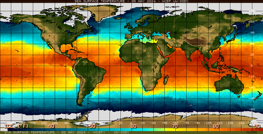
Are anomalous cold sea surface temperatures in the North Atlantic bringing cold temperatures to northern Europe?

Have a look now -- I didn't manage to save the image from last week, and the hotter waters along the East Coast of the U.S. have pushed northeast, but colder waters are still in the way.

http://earth.nullschool.net/#current/ocean/surface/currents/overlay=sea_surface_temp_anomaly/orthographic=-31.37,45.10,881

On November 18, 2014:


LEGEND OF UNOFFICIAL RECORDS:


Daily Close

Daily Tied
.
Daily Broken

Monthly
Tied/Broken

All-time
Tied/Broken
HIGH
##.#
##.#
.
##.#

##.#

##.#
LOW
##.#
##.#
.
##.#

##.#

##.#
IDCityCountry
Current
Temp.
(°F)

Unofficial Daily /
Monthly / Alltime
Record (°F)

Margin of
Unofficial Daily
Record (°F)

Year of Unofficial
Daily / Monthly /
Alltime Record

Database
Length
(years)
ID
KPSCPasco, WAUnited States
99.0

 95.0   107.1   117.0

+4.0

2003  2008  2008

44
KPSC
KMWHMoses Lake, WAUnited States
96.1

 93.0   106.0   111.9

+3.0

1989  1949  2002

62
KMWH
KSHNShelton, WAUnited States
82.0

 79.0    97.0   104.0

+3.0

2009  2012  2001

39
KSHN
KGEGSpokane, WAUnited States
91.0

 88.0   100.9   106.0

+3.0

1952  1985  1954

72
KGEG
KEATWenatchee, WAUnited States
93.9

 91.0   104.0   108.0

+2.9

2003  1983  1995

42
KEAT
CYXCCranbrook, B. C.Canada
84.2

 82.2   100.8   100.8

+2.0

1989  1984  1984

38
CYXC
YGELGeraldton AirportAustralia
80.6

 79.0    94.5   118.0

+1.5

1949  2006  1980

73
YGEL
KSKAFairchild AFB, WAUnited States
87.1

 86.0    97.9   104.4

+1.0

2003  1993  1986

75
KSKA
KALWWalla Walla, WAUnited States
95.0

 93.9   106.9   113.0

+1.0

1955  1987  2002

67
KALW
ZSAMXiamenChina
93.2

 93.2   111.2   111.2

0.0

2012  1994  1994

51
ZSAM
RORSShimoji-Shima IslandJapan
87.8

 87.8    91.4    95.0

0.0

2013  1982  1985

35
RORS
RCSSSungshan / TaipeiTaiwan
95.0

 95.0   100.4   104.0

0.0

2009  1949  1957

61
RCSS
KYKMYakima, WAUnited States
95.0

 95.0   105.1   109.0

0.0

1948  1993  1948

67
KYKM
KSFFSpokane, WAUnited States
88.0

 88.0   100.9   104.0

0.0

2003  1993  1973

42
KSFF
KHIOPortland, ORUnited States
84.0

 84.0   102.0   108.0

0.0

1982  2001  1999

37
KHIO
CYHEHope, B. C.Canada
80.6

 80.6    94.1   102.2

0.0

1995  1979  1979

38
CYHE
CYCGCastlegar AirportCanada
86.0

 86.0   100.4   104.0

0.0

1992  1981  1982

38
CYCG
CYCDNanaimo AirportCanada
80.6

 80.6    93.2    98.6

0.0

2002  1984  2012

38
CYCD
SPMETumbesPeru
89.6

 90.0   104.0   104.9

-0.4

1997  1977  1989

41
SPME
KPUWPullman / Moscow, WAUnited States
80.1

 81.0    97.0   102.9

-0.9

2003  1985  2002

42
KPUW
KPDTPendleton, ORUnited States
91.9

 93.0   107.1   111.9

-1.0

1955  1973  2002

77
KPDT
KPWTBremerton National, WAUnited States
78.8

 79.9    95.0   104.0

-1.1

1995  1996  2001

42
KPWT
VHHHHong Kong Inter-National AirportHong Kong
91.4

 92.7    98.6   100.9

-1.3

2011  1997  2006

42
VHHH
ROMYMiyakojimaJapan
87.8

 89.1    93.2   102.2

-1.3

2013  1982  1977

42
ROMY
YSSYSydney AirportAustralia
73.4

 74.8   100.4   114.8

-1.3

1995  1964  1949

76
YSSY
YSRIRichmond Aus-AfbAustralia
69.8

 71.6    79.2   114.8

-1.8

2005  1954  2010

61
YSRI
WAJJJayapura / SentaniIndonesia
91.4

 93.2   100.4   114.8

-1.8

2007  1996  1957

42
WAJJ
CYRVRevelstoke, B. C.Canada
84.2

 86.0    98.6   100.4

-1.8

1958  2009  1980

41
CYRV
KRBGRoseburg, ORUnited States
93.0

 95.0   105.1   108.0

-2.0

1955  1993  1963

60
KRBG
KLWSLewiston, IDUnited States
91.0

 93.0   105.1   115.0

-2.0

1983  1949  1948

67
KLWS
PKWAKwajaleinMarshall Islands
87.6

 90.0    91.9   103.5

-2.4

1953  1984  1985

71
PKWA
ZGOWShantouChina
91.4

 93.9   107.6   107.6

-2.5

2013  2000  2000

51
ZGOW
PKMRMajuro Atoll NWS OfficeMarshall Islands
87.1

 89.6   108.0   122.0

-2.5

2012  1983  1994

65
PKMR
YBBNBrisbane Airport M. OAustralia
75.2

 77.9    87.8   104.4

-2.7

2001  1971  1972

69
YBBN
YWLMWilliamtown AirportAustralia
73.4

 76.3    79.2   112.6

-2.8

1995  1944  2010

69
YWLM
KMFRMedford, ORUnited States
97.0

100.0   111.0   113.9

-3.0

1955  1993  1985

67
KMFR
KLMTKlamath Falls, ORUnited States
88.0

 91.0   102.9   102.9

-3.0

2013  1983  1983

55
KLMT
.
EBBRBruxelles NationalBelgium
44.6

 41.7    33.8     1.2

+2.9

1985  1980  1982

53
EBBR
TNCAQueen Beatrix AirportAruba
80.6

 77.7    69.8    61.5

+2.8

1990  1979  1994

45
TNCA
EGXCConingsby Royal AFBUnited Kingdom
41.0

 38.3    30.0     8.2

+2.7

1989  1993  2012

49
EGXC
EGUNMildenhall Royal AFBUnited Kingdom
42.6

 39.9    30.9     5.0

+2.7

1967  1962  1963

39
EGUN
EGYMMarhamUnited Kingdom
39.2

 36.7    30.9    -7.6

+2.5

2001  1989  1979

45
EGYM
EGXULinton-On-OuseUnited Kingdom
39.2

 36.7    33.8     1.4

+2.5

1989  1989  1979

42
EGXU
EGVAFairford Royal AFBUnited Kingdom
43.5

 41.0    34.3    -2.2

+2.5

1974  1962  1982

56
EGVA
EGXPScamptonUnited Kingdom
41.0

 39.0    33.4     3.9

+2.0

2001  1991  2010

37
EGXP
SBBVBoa Vista, Boa Vista IntlBrazil
73.4

 71.6    53.6    53.6

+1.8

1974  1973  1973

42
SBBV
DNKNKanoNigeria
73.4

 71.6    48.2    39.2

+1.8

2013  2002  1980

35
DNKN
MUCMCamaguey AeropuertoCuba
69.8

 68.0    55.9    32.0

+1.8

1974  1974  2009

47
MUCM
LGSYSkirosGreece
59.0

 57.2    49.6    23.0

+1.8

2006  2002  1975

48
LGSY
ETNHHohnGermany
39.2

 37.4    33.8    -9.4

+1.8

1991  2009  1981

37
ETNH
ETHBBueckeburgGermany
42.8

 41.0    33.8    -7.1

+1.8

1985  1977  1997

42
ETHB
ENMLMolde / AroNorway
44.6

 42.8    32.0    -4.0

+1.8

1984  1986  1978

39
ENML
ESCFLinkoping / MalmenSweden
39.2

 37.6    31.3   -20.0

+1.6

2001  2009  2010

38
ESCF
EGYDCranwellUnited Kingdom
41.0

 40.1    35.6     8.2

+0.8

2001  1975  1985

48
EGYD
ESSPNorrkopingSweden
37.4

 37.4    30.2   -20.2

0.0

1990  2009  1979

39
ESSP
EINNShannon AirportIreland
41.0

 41.0    33.8    11.7

0.0

1977  1989  2010

42
EINN
EGNJHumbersideUnited Kingdom
44.6

 44.6    37.4     6.8

0.0

1984  1991  2010

37
EGNJ
EDDHHamburg-FuhlsbuettelGermany
39.2

 39.9    33.8   -20.0

-0.6

1951  1975  1940

54
EDDH
ENRORoros LufthavnNorway
32.0

 33.8    24.8   -47.2

-1.8

2010  2011  1987

36
ENRO
ESSVVisby FlygplatsSweden
37.4

 40.3    31.5    -9.9

-2.9

2005  1991  1985

42
ESSV
EIDWDublin AirportIreland
33.8

 38.1    35.8    10.0

-4.3

1999  2001  2010

42
EIDW
IDCityCountry
Current
Temp.
(°F)

Unofficial Daily /
Monthly / Alltime
Record (°F)

Margin of
Unofficial Daily
Record (°F)

Year of Unofficial
Daily / Monthly /
Alltime Record

Database
Length
(years)
ID
LEGEND OF UNOFFICIAL RECORDS:
Daily Close
Daily Tied
.
Daily Broken
Monthly
Tied/Broken
All-time
Tied/Broken
HIGH
##.#
##.#
.
##.#
##.#
##.#
LOW
##.#
##.#
.
##.#
##.#
##.#
http://www.coolwx.com/record/

Sunday, August 24, 2014

RUSSIAN RIVER WATER UNEXPECTED CULPRIT BEHIND ARCTIC FRESHENING

Russian river water unexpected culprit behind Arctic freshening

by Sandra Hines, UW Today, January 4, 2012

A hemisphere-wide phenomenon – and not just regional forces – has caused record-breaking amounts of freshwater to accumulate in the Arctic's Beaufort Sea.


Frigid freshwater flowing into the Arctic Ocean from three of Russia's mighty rivers was diverted hundreds of miles to a completely different part of the ocean in response to a decades-long shift in atmospheric pressure associated with the phenomenon called the Arctic Oscillation, according to findings published in the January 5, 2012, issue of Nature.
The new findings show that a low pressure pattern created by the Arctic Oscillation from 2005 to 2008 drew Russian river water away from the Eurasian Basin, between Russia and Greenland, and into the Beaufort Sea, a part of the Canada Basin bordered by the United States and Canada. It was like adding 10 feet (3 meters) of freshwater over the central part of the Beaufort Sea.
“Knowing the pathways of freshwater in the upper ocean is important to understanding global climate because of freshwater's role in protecting sea ice – it can help create a barrier between the ice and warmer ocean water below – and its role in global ocean circulation. Too much freshwater exiting the Arctic would inhibit the interplay of cold water from the poles and warm water from the tropics,” said Jamie Morison, an oceanographer with the University of Washington's Applied Physics Laboratory and lead author of the Nature paper.

Red arrows show the new path of Russian river water into the Canada Basin. The previous freshwater pathway – across the Eurasian Basin toward Greenland and the Atlantic – was altered by atmospheric conditions created by the Arctic Oscillation. Credit: University of Washington
Morison and his six co-authors from the UW and NASA's Jet Propulsion Laboratory are the first to detect this freshwater pathway and its connection to the Arctic Oscillation. The work is based on water samples gathered in the field combined with satellite oceanography possible for the first time with data from NASA satellites known as ICESat and GRACE.
“Changes in the volume and extent of Arctic sea ice in recent years have focused attention on the impacts of melting ice,” said co-author Ron Kwok, senior research scientist with the Jet Propulsion Laboratory in Pasadena, Calif. “The combined GRACE and ICESat data allow us to now examine the impacts of widespread changes in ocean circulation.”

Red arrows show the new path of Russian river water into the Canada Basin. The previous freshwater pathway – across the Eurasian Basin toward Greenland and the Atlantic – was altered by atmospheric conditions created by the Arctic Oscillation. Credit: University of Washington
Taken as a whole, the salinity of the Arctic Ocean is similar to the past, but the change in the freshwater pathway means the Eurasian Basin has gotten more saline while the Canada Basin has gotten fresher.
“The freshening on the Canadian side of the Arctic over the last few years represents a redistribution of freshwater, there does not seem to be a net freshening of the ocean,” Kwok said.
In the Eurasian Basin, the change means less freshwater enters the layer known as the cold halocline and could be contributing to declines in ice in that part of the Arctic, Morison said. The cold halocline normally sits like a barrier between ice and warm water that comes into the Arctic from the Atlantic Ocean. Without salt the icy cold freshwater is lighter, which is why it is able to float over the warm water.
In the Beaufort Sea, the water is the freshest its been in 50 years of record keeping, he said. The new findings show that only a tiny fraction is from melting ice and the vast majority is Eurasian river water.
The Beaufort Sea stores a significant amount of freshwater from a number of sources, especially when an atmospheric condition known as the Beaufort High causes winds to spin the water in a clockwise gyre. When the winds are weaker or spin in the opposite direction, freshwater is released back into the rest of the Arctic Ocean, and from there to the worlds oceans. Some scientists have said a strengthening of the Beaufort High is the primary cause of freshening, but the paper says salinity began to decline in the early 1990s, a time when the Beaufort High relaxed and the Arctic Oscillation increased.
“We discovered a pathway that allows freshwater to feed the Beaufort gyre,” Kwok said. “The Beaufort High is important but so are the broader-scale effects of the Arctic Oscillation.”
“A number of people have come up with ways of looking at regional forces at work in the Arctic,” Morison said, “To better understand changes in sea ice and the Arctic overall we need to look more broadly at the hemisphere-wide Arctic Oscillation, its effects on circulation of the Arctic Ocean and how global warming might enhance those effects.”
In coming years if the Arctic Oscillation stops perpetuating that low pressure, the freshwater pathway should switch back.
Morison and the co-authors argue that, compared to prior years, the Arctic Oscillation has been in its current state for the last 20 years. For example, the changes detected in response to the Arctic Oscillation between 2005 and 2008 are very similar to freshening seen in the early 1990s, Morison said.
Discerning the track of freshwater from Eurasian rivers would have been impossible without the ICESat and GRACE satellites, Kwok and Morison agree. With satellite measurements of ocean height and bottom pressures, the researchers could separate the changes in mass from changes in density – or freshwater content – of the water column.
“To me its pretty spectacular that you have these satellites zipping around hundreds of kilometers above the Earth and they give us a number about salinity that's very close to what we get from lowering little sampling bottles into the ocean,” Morison said.
Other co-authors are Cecilia Peralta-Ferriz with the UWs School of Oceanography and Matt Alkire, Ignatius Rigor, Roger Andersen and Mike Steele, all with the UWs Applied Physics Laboratory. The work was funded by the National Science Foundation and NASA. For more information: Morison, 206-543-1394 (office), 206-310-5307 (cell), morison@apl.washington.edu and Kwok, contact via Alan Buis, 818-354-0474, alan.d.buis@jpl.nasa.gov
Top Image: Julian Olden and graduate student Thomas Pool weigh invasive carp from an Arizona stream. Credit: Olden Lab

Monday, November 4, 2013

Stefan Rahmstorf: The Thermohaline Ocean Circulation

A Brief Fact Sheet by Stefan Rahmstorf

For an updated and more detailed version, see the following paper (pdf, 3MB):

Rahmstorf, S., 2006: Thermohaline Ocean Circulation. In: Encyclopedia of Quaternary Sciences, Edited by S. A. Elias. Elsevier, Amsterdam. 

 realclimate
 KlimaLounge


Books: (click on image)


692,470 visitors
since 5 Jan 2009


Atlantic ocean currents

What is the thermohaline circulation (THC)?

As opposed to wind-driven currents and tides (which are due to the gravity of moon and sun), the thermohaline circulation (Fig. 1)  is that part of the ocean circulation which is driven by density differences. Sea water density depends on temperature and salinity, hence the name thermo-haline. The salinity and temperature differences arise from heating/cooling at the sea surface and from the surface freshwater fluxes (evaporation and sea ice formation enhance salinity; precipitation, runoff and ice-melt decrease salinity). Heat sources at the ocean bottom play a minor role.
 

Figure 1. Schematic representation of the global thermohaline circulation.
Surface currents are shown in red, deep waters in light blue and bottom waters in dark blue. The main deep water formation sites are shown in orange. (After [1], modified by S.R.)
    
In contrast to the wind-driven currents, the THC is not confined to surface waters but can be regarded as a big overturning of the world ocean, from top to bottom. The thermohaline circulation consists of:
  • Deep water formation: the sinking of water masses, closely associated with (but not to be confused with) convection, which is a vertical mixing process, [2]). Deep water formation takes place in a few localised areas: the Greenland-Norwegian Sea, the Labrador Sea, the Mediteranean Sea, the Wedell Sea, the Ross Sea.
  • Spreading of deep waters (e.g., North Atlantic Deep Water, NADW, and Antarctic Bottom Water, AABW), mainly as deep western boundary currents (DWBC).
  • Upwelling of deep waters: this is not as localised and difficult to observe. It is thought to take place mainly in the Antarctic Circumpolar Current region, possibly aided by the wind (Ekman divergence).
  • Near-surface currents: these are required to close the flow. In the Atlantic, the surface currents compensating the outflow of NADW range from the Benguela Current off South Africa via Gulf Stream and North Atlantic Current into the Nordic Seas off Scandinavia (Fig. 2). (Note that the Gulf Stream is primarily a wind-driven current, as part of the subtropical gyre circulation. The thermohaline circulation contributes only roughly 20% to the Gulf Stream flow.)


Figure 2. Thermohaline circulation of the Atlantic. 
This highly simplified cartoon of Atlantic currents shows warmer surface currents (red) and cold north Atlantic Deep Water (NADW, blue). The thermohaline circulation heats the North Atlantic and Northern Europe. It extends right up to the Greenland and Norwegian Seas, pushing back the winter sea ice margin. (From [3].)

Some observational data

The volume transport of the overturning circulation at 24 N has been estimated from hydrographic section data ([4]) as 17 Sv (1 Sv = 106 m3/s), its heat transport as 1.2 PW (1 PW = 1015 W). More recently, an inverse model by [5] yielded 15+/-2 Sv NADW overturning in the high latitudes. (Note: when comparing these numbers with models care needs to be taken what exactly is compared - in models, the most common measure of NADW overturning is the maximum of the zonally integrated transport stream function in the North Atlantic, sometimes also the outflow value at 30 S.)


What drives the THC?

The short answer would be: high-latitude cooling. In cold regions the highest surface water densities are reached, this causes convective mixing and sinking of deep water, which drives the circulation.

Reality is more complex. Pressure gradients at depth, resulting from density gradients in the overlying waters, are the driving force in the equations of motion. As the density forcing occurs at the surface (see above), a subtle question is why the density differences and the circulation affect the whole ocean depth and are not confined to a near-surface layer. [6] showed that a deep circulation only arises when heating (buoyancy source) is at depth and cooling at the surface. The reason that there is a deep circulation after all is turbulent mixing, which brings down the heat on a time scale of ~1,000 years. It has been shown that in the long-term equilibrium the strength of the thermohaline circulation in models depends on the turbulent mixing coefficient [7], and that the energy required for this turbulent mixing comes to a large extent from the moon via tidal currents ([8]).


This discussion can be labelled: is the THC pushed or pulled ([9])? I.e., pushed by formation of cold deep water, or pulled by downward diffusion of heat through the thermocline? The answer is a question of time scale: ultimately, in the long run, it is pulled. But on shorter time scales, up to centuries, it can be considered pushed in the sense that it is density changes in the deep water formation regions which affect the circulation strength. If this density drops too much so that deep water formation is not possible, the circulation stops. Ultimately, on the long time scale of turbulent mixing, the deep ocean density will drop as well until new deep water formation can start.


Non-linear behaviour of the THC

As mentioned above, highest surface densities in the world ocean are reached where water is very cold, while lower densities are found in the saltier but warmer tropical and subtropical areas. In this sense the THC is thermally driven. Nevertheless, the influence of salinity is important and is what causes the non-linearity of the system. This was first described in a classic paper by [10] with the help of a simple box model. Salinity is involved in a positive feedback: higher salinity in the deep water formation area enhances the circulation, and the circulation in turn transports higher salinity waters into the deep water formation regions (which tend to be regions of net precipitation, i.e., freshwater would accumulate and surface salinity would drop if the circulation stopped). Put simply, in Stommel's model the high-latitude salinity increases linearly with the flow, and the flow increases linearly with high-latitude salinity, which combined gives a quadratic (i.e., non-linear) equation. This leads to two possible equilibrium states, the system is bistable in a certain parameter range. This becomes more than an academic point as complex circulation models behave in the same way, and as the present North Atlantic in many models is in the bistable regime ([11]). The first coupled climate model to show these two equilibria  (discovered quite by accident) is the one by [12].

The situation can be described with a simple stability diagram showing strength of the THC as a function of the freshwater input into the North Atlantic. This shows the bistable regime and a saddle-node bifurcation point where the circulation breaks down. It is discussed in more detail (but for the non-specialist) in [13].


An important point is that the salt transport feedback is not the only feedback rendering the system non-linear. The convective mixing process is itself a highly non-linear, self-sustaining process. In models this can lead to multiple stable convection patterns ([14, 15]), which on one hand can cause artefacts related to the coarse model grid. On the other hand this may be part of a real mechanism for shifts in convection location, as have apparently occured during glacial times.


The bottom line is: salinity leads to non-linearity which causes the existence of multiple equilibria and thresholds in the THC.


A related question is: why is no deep water formed in the North Pacific? Salinity there is too low, but why? A body of literature exists on this topic; it is discussed, e.g., in [16]. My opinion is: for geographical reasons so much freshwater enters the North Pacific that it is far in the monostable regime where no deep water formation is possible.


The effect on climate

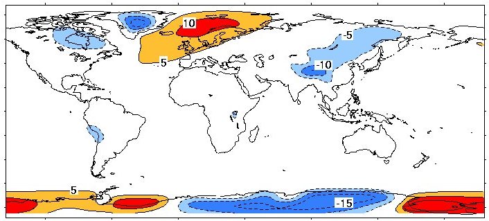
The climatic effect of the THC is still to some extent under discussion, and is due to the heat transport of ~1 PW of this circulation. Back-of-the-envelope calculations suggest that this amount of heat transported into the northern North Atlantic (north of 24 N) should warm this region by ~5K. This is indeed roughly the difference between sea surface temperature (SST) in the North Atlantic as compared to the North Pacific at similar latitudes. A look at sea ice margins suggest that they are pushed back by the warm surface currents in the Atlantic sector as compared to the North Pacific (Fig. 1), this in turn leads to reduced reflection of sunlight and thus warming (albedo feedback). A look at global surface air temperatures is also quite suggestive: over the three main deep water formation regions of the world ocean, air temperatures are warmer by up to ~10K compared to the latitudinal mean.

These observations are, however, no quantitative proof of the climatic effect of the THC, and other explanations can be invoked, such as planetary waves in the atmosphere, locked in place by the geography (Rocky mountains).


One way to estimate the effect of the THC is to switch it off in coupled climate models (by adding a lot of freshwater to the northern Atlantic), and compare the surface climate before and after switching it off. Roughly, this leads to a cooling with a maximum of ~10K over the Nordic Seas (e.g., [12, 17]). The maximum tends to occur near the sea ice margin due to the ice albedo effect. Unfortunately, the details of this cooling are model-dependent: one model shows cooling up to 22K  in annual mean and 33K in winter ([18]). Models also differ in how widespread the cooling is: most tend to affect temperatures over land in  northwestern Europe (Scandinavia, Britain) by several degrees, others show strong cooling further west affecting Canada ([19]).
 

Figure 3. Deviation of surface air temperature from zonal mean.
Deviations are shown in degree C. Based on NCAR surface air temperature climatology, reproduced from [20].


History of the THC

Sediment data document that the THC has undergone major changes in the history of climate (e.g., [21, 22]). Three major circulation modes were indentified: a warm mode similar to the present-day Atlantic, a cold mode with NADW forming south of Iceland in the Irminger Sea, and a switched-off mode ([23]). The latter appears to have occurred after major input of freshwater, either from surging glacial ice sheets (Heinrich events) or in form of meltwater floods (e.g., Younger Dryas event). The most dramatic climate events recorded in Greenland, the Dansgaard-Oeschger (D/O) events, were probably associated with north-south shifts in convection location, i.e. transitions between warm and cold modes of the Atlantic THC. Recent simulations of such shifts show encouraging agreement with paleoclimatic data ([24]).


The THC in anthropogenic global warming

Global warming can affect the THC in two ways: surface warming and surface freshening, both reducing the density of high-latitude surface waters and thus inhibiting deep water formation. [25] was the first to warn that this could lead to a breakdown of the THC and to abrupt climate change. Subsequently, [26, 27] showed that this could indeed occur for strong global warming (i.e., for a quadrupling, but not for a doubling of CO2). In these scenarios there was no surface cooling, as the high CO2 levels more than compensated for the reduced ocean heat transport. The possibility of a real cooling (both a relative cooling, i.e. a drop back to roughly pre-industrial temperatures after an initial warming phase, and in the longer run an absolutecooling below preindustrial values) as a result of anthropogenic warming was first demonstrated in a sensitivity study by [20]. Significant absolute cooling can arise after COlevels decline, but the THC remains switched off after its collapse is triggered in a rapid warming phase.

A THC collapse is now widely discussed as one of a number of "low probability - high impact" risks associated with global warming. More likely than a breakdown of the THC, which only occurs in very pessimistic scenarios, is a weakening of the THC by 20-50%, as simulated by many coupled climate models ([28]). 
Key open questions include:
  • What changes in freshwater input to the North Atlantic will result from global warming? (Uncertainty e.g. due to uncertain estimates of Greenland meltwater runoff, ignored so far in most models, and due to possible changes in ENSO ([29]).)
  • What is the risk of exceeding a threshold for THC collapse for a given warming?
  • What other thresholds exist? (e.g., a local shutdown of convection in the Labrador Sea as simulated by [30], rather than a full THC collapse.)
  • What consequences would result for marine ecosystems?
  • How would temperatures over land be affected by a collapse scenario? (Just a reduced warming, or a warming followed by abrupt cooling?)