Ice-cliff failure via retrogressive slumping doi.org/10.1130/G45880.1

Geology, (2019) ; https://doi.org/10.1130/G45880.1

Ice-cliff failure via retrogressive slumping

Byron R. Parizek, 

Knut Christianson, 

Richard B. Alley, 

Denis Voytenko, 

Irena Vaňková, 

Timothy H. Dixon, 

Ryan T. Walker, and 

David M. Holland

Abstract

Retrogressive slumping could accelerate sea-level rise if ice-sheet retreat generates ice cliffs much taller than observed today. The tallest ice cliffs, which extend roughly 100 m above sea level, calve only after ice-flow processes thin the ice to near flotation. Above some ice-cliff height limit, the stress state in ice will satisfy the material-failure criterion, resulting in faster brittle failure. New terrestrial radar data from Helheim Glacier, Greenland, suggest that taller sub-aerial cliffs are prone to failure by slumping, unloading submarine ice to allow buoyancy-driven full-thickness calving. Full–Stokes diagnostic modeling shows that the threshold cliff height for slumping is likely slightly above 100 m in many cases and roughly twice that (145–285 m) in mechanically competent ice under well-drained or low-melt conditions.

https://pubs.geoscienceworld.org/gsa/geology/article/569567/ice-cliff-failure-via-retrogressive-slumping

Sea Levels To Rise More Than Expected Due To Warming-Driven Surge In Greenland Ice Loss

by Joe Romm and Jeff Spross, Climate Progress, March 17, 2014

Greenland’s contribution to global sea level has soared in the past two decades. An important new study finds that the massive northeastern part of the ice sheet, previously thought to be stable, has begun shedding ice. If this trend continues — and researchers say “a self-perpetuating feedback process may have been triggered” — actual sea level rise this century will likely be higher than many current models had projected.

Covering 660,000 square miles — roughly 80% of the country — Greenland’s ice sheet is second only in size to Antarctica’s. Scientists estimate that melting from the ice sheet as a whole has accounted for about 16% of sea level rise every year for the last two decades.

Research had also long suggested the northeastern portion of the ice sheet was stable. As a result, it was largely left out of the models used to anticipate future sea level rise.

But the new study, “Sustained mass loss of the northeast Greenland ice sheet triggered by regional warming,” published in Nature Climate Change (subs. req’d), suggests the northeastern portion began melting rapidly around 2003. And after first jumping from an ice loss rate of zero to about 10 billion metric tons per year, it’s now approaching 15 or 20 billion metric tons per year and may well keep accelerating.

“Most projections of the future behaviour of the ice sheet have no, or little, contribution from this part of Greenland,” said Professor Jeremy Bamber of Bristol University, a co-author of the study. “But these new results suggest that this region is sensitive to changes in climate and has the potential to contribute significantly now and in the future.”

The team arrived at their conclusion using a combination of surface elevation data from airplanes and four different satellites, along with a GPS-linked network of 50 stations located along the coast of Greenland’s ice sheet. The overall collection of data spanned 1978 to 2012 and was used to essentially weigh the ice sheet’s mass.

Specifically, the study suggests a series of particularly warm summers leading up to 2003 — bringing higher temperatures in both the atmosphere and the surrounding ocean — triggered the speed up in melting.

Much of the ice melt was also historically held in check by an ice barrier at the coast, which itself is now melting as well, allowing the entire system to speed up. Coauthor Prof. Kurt Kjær explains that there was “a clear acceleration in loss of mass after 2006.” He warns:

“This acceleration has since continued and even increased. The increased loss of mass can be explained by a combination of warmer air in the summer and a rise in sea temperatures. This has reduced the extent of sea ice, which otherwise helps to stabilize the glaciers. Our results also demonstrate that after 2009 both air and, in particular, sea temperatures have returned to the level from before 2006. At the same time, the sea ice has maintained its previous extent, although the loss in mass has increased even further. This indicates that a self-perpetuating feedback process may have been triggered….”

The loss of Arctic sea ice creates a well-known amplifying feedback whereby white ice is replaced by the dark blue sea, which absorbs far more sunlight and hence far more solar energy. Back in 2011, scientists warned that the Greenland ice sheet “could undergo a self-amplifying cycle of melting and warming“ that is “difficult to halt.” A 2012 study found we may be close to a “tipping point” in which “the summer melt area covers the entire land mass.”

Another cause for concern is Greenland’s ice streams. These are essentially “rivers” of ice that drain ice sheets in much the same way networks of streams and rivers drain water from huge areas on land. And the drainage basin for Greenland’s northeast portion is enormous — covering 16% of the ice sheet and reaching 373 miles inland, all the way to the center of the country.

Regional warming has triggered rapid ice loss in a vast portion of the northeastern Greenland Ice Sheet (NEGIS). Red indicates the fastest melting. (Via Ohio State)

“This implies that changes at the margin can affect the mass balance deep in the center of the ice sheet,” said Shfaqat Abbas Khan, a senior researcher at the National Space Institute at the Technical University of Denmark, and the leader of the research team. “Furthermore, due to the huge size of the northeast Greenland ice stream, it has the potential of significantly changing the total mass balance of the ice sheet in the near future.”

In short, the research adds to the case that actual sea level rise in the future will be on the high end of the projections from the Intergovernmental Panel on Climate Change — which ranged from one to three feet by the end of the century. Other climate scientists have projected even higher numbers.

Most climate scientists and glaciologists that Climate Progress has spoken to in recent years have said humanity should plan for at least three feet of sea level rise this century — and considerably more than that if we stay on our current high-end emissions path.

http://thinkprogress.org/climate/2014/03/17/3411561/sea-levels-greenland-ice-loss/

NASA data shed new light on changing Greenland ice

by George Hale, phys.org, March 10, 2014

This is the calving front of Greenland's Jakobshavn Glacier seen during an IceBridge survey flight in 2012. Credit: NASA / Jefferson Beck

Research using NASA data is giving new insight into one of the processes causing Greenland's ice sheet to lose mass. A team of scientists used satellite observations and ice thickness measurements gathered by NASA's Operation IceBridge to calculate the rate at which ice flows through Greenland's glaciers into the ocean. The findings of this research give a clearer picture of how glacier flow affects the Greenland Ice Sheet and shows that this dynamic process is dominated by a small number of glaciers.

Over the past few years, Operation IceBridge measured the thickness of many of Greenland's glaciers, which allowed researchers to make a more accurate calculation of ice discharge rates. In a new study published in the journal Geophysical Research Letters, researchers calculated ice discharge rates for 178 Greenland glaciers more than one kilometer (0.62 miles) wide.

Ice sheets grow when snow accumulates and is compacted into ice. They lose mass when ice and snow at the surface melts and runs off and when glaciers at the coast discharge ice into the ocean. The difference between yearly snowfall on an ice sheet and the sum of melting and discharge is called a mass budget. When these factors are equal, the mass budget is balanced, but for years the Greenland Ice Sheet has had a negative mass budget, meaning the ice sheet is losing mass overall.

For years the processes of surface melt and glacier discharge were roughly equal in size, but around 2006 surface melt increased and now exceeds iceberg production. In recent years, computer model projections have shown an increasing dominance of surface melt, but a limited amount of glacier thickness data made pinpointing a figure for ice discharge difficult.

Ice discharge is controlled by three major factors: ice thickness, glacier valley shape and ice velocity. Researchers used data from IceBridge's ice-penetrating radar – the Multichannel Coherent Radar Depth Sounder, or MCoRDS, which is operated by the Center for Remote Sensing of Ice Sheets at the University of Kansas, Lawrence, Kan. – to determine ice thickness and sub-glacial terrain, and images from satellite sources such as Landsat and Terra to calculate velocity. The team used several years of observations to ensure accuracy. "Glacier discharge may vary considerably between years," said Ellyn Enderlin, glaciologist at the University of Maine, Orono, Maine and the study's lead author. "Annual changes in speed and thickness must be taken into account."

Being able to study Greenland in such a large and detailed scale is one of IceBridge's strengths. "IceBridge has collected so much data on elevation and thickness that we can now do analysis down to the individual glacier level and do it for the entire ice sheet," said Michael Studinger, IceBridge project scientist at NASA's Goddard Space Flight Center in Greenbelt, Md. "We can now quantify contributions from the different processes that contribute to ice loss."

With data on glacier size, shape and speed, researchers could calculate each glacier's contribution to Greenland's mass loss and the total volume of ice being discharged from the Greenland Ice Sheet. Of the 178 glaciers studied, 15 accounted for more than three-quarters of ice discharged since 2000, and four accounted for roughly half. Considering the large size of some of Greenland's glacier basins, such as the areas drained by the Jakobshavn, Helheim and Kangerdlugssuaq glaciers, this was not exactly surprising.

What they also found was that the size of these basins did not necessarily correlate with glacier discharge rate, shuffling the order of Greenland's largest glaciers. Previously Helheim Glacier was thought to be Greenland's third largest glacier, but this study puts it in fifth place and adds two southeast Greenland glaciers, Koge Bugt and Ikertivaq South to the list of big ice-movers.

Glacier thickness measurements and this study's calculation methods have the potential to improve future computer model projections of the Greenland Ice Sheet. And with a new picture of which glaciers contribute most to mass loss, IceBridge will be able to more effectively target areas in future campaigns, promising more and better data to add to the research community's body of knowledge.

 Explore further: Mathematician uses skills to study Greenland's retreating glaciers (w/ Video)

Journal reference: Geophysical Research Letters  

Provided by NASA's Goddard Space Flight Center

http://phys.org/news/2014-03-nasa-greenland-ice.html

D. Bailey & M. Pelto: Zebras? In Greenland? Really? [Variations in Greenland Ice Sheet outlet glacier behavior]

Zebras? In Greenland? Really?

by Daniel Bailey and Mauri Pelto, Skeptical Science, April 11, 2012

At first glance, zebras are all the same.  Sure, you can argue that they are black with white stripes or white with black stripes.  But nobody really cares; they're zebras, after all.

[sorry, readers, in the interest of saving space the photo of the zebras is not posted -- but I am sure you will have no trouble imagining them]

Just as each zebra has an individualized set of stripes, making them unique, so also are each of the individual glaciers in Greenland unique.  They each have varied lengths, heights, widths, fjord geometries, differently-sized accumulation zones (where they "pack on weight") and flow speeds.  Each is located in a different part of Greenland and thus are also affected differently by their latitude, oceanic currents (for the marine-terminating glaciers), weather and climatic patterns.  And also by the modifying effects of Arctic amplification of the warming of the globe.

Variations in Greenland Ice Sheet outlet glacier behavior

The Greenland Ice Sheet has an area of 2.17 million square kilometers (1.28 million square miles) and spans 18 degrees of latitude from north to south.  It is not surprising that over this vast area that the geology and climate vary substantially and that this leads to variations in behavior of Greenland glaciers.  Our tendency is to lump the Greenland Ice Sheet into one category impacted similarly by each of the dynamic forces that impact flow. This is akin to saying banks, credit unions and savings and loan institutions are impacted similarly by all the economic forces.  In the case of a recession there is a shared signal, just as with global warming there is a shared signal amongst Greenland glaciers.   This is a simplification that does not work.  In this article we divide the glaciers into four main categories to illustrate the different properties and sensitiveness of each.

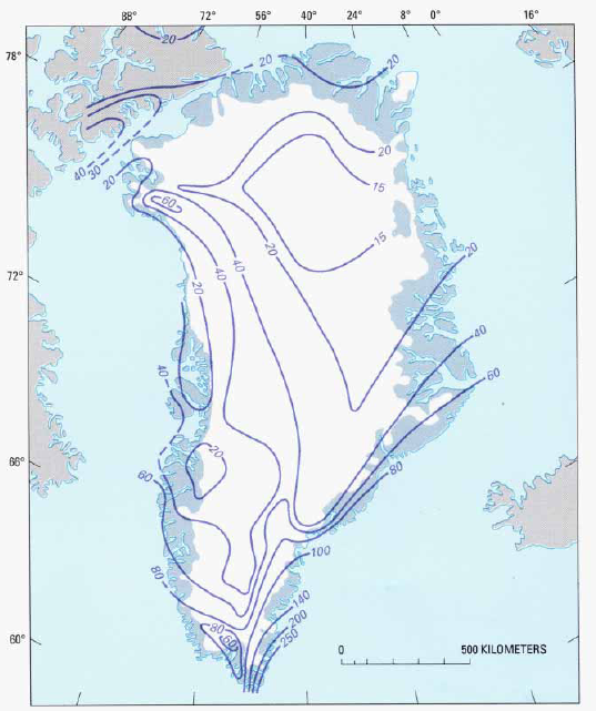
The surface mass balance of the glacier is the difference of accumulating snow on the ice sheet (its income) and snow and ice losses from melting and calving (its expenditures).  The volume of the ice sheet is its asset.  On an ice sheet, the main factor driving flow is simply the mass balance input in the accumulation zone.  The higher the accumulation rate the faster the movement; the accumulated snow is inexorably moved downslope towards the ocean and the margin of the ice sheet.  Observation of a precipitation map (focused not on the outer margin, but on the accumulation zone of the ice sheet) indicates that highest accumulation rates, over 40 cm per year, extend along the western side of the ice sheet to the southeast quadrant of the ice sheet.  

Figure 2. Distribution of precipitation in Greenland (in grams per square centimeter per year). Contours dashed where inferred. Ice-free areas are shown in dark gray. (USGS Satellite Image Atlas of Greenland)

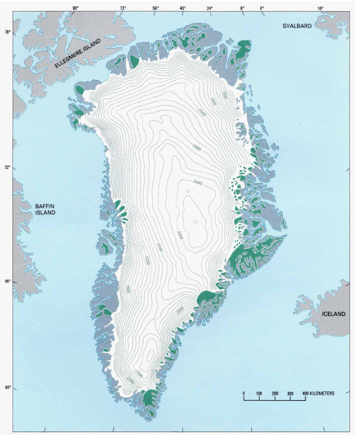
The overall topography of the ice sheet is controlled both by the basal and peripheral geology and the mass balance distribution of the ice sheet.  The higher rates of mass accumulation inland and the greater melting nearer the margin yield a steeper profile for the ice sheet. 

Figure 3. Topographic map of the Greenland ice sheet. The contour interval is 100 m. Local ice caps and ice domes are shown in green. Ice-free areas are shown in dark gray. (USGS Satellite Image Atlas of Greenland)

Figure 3 shows that the contours have the closest spacing along the west margin and in the southeast, just as the high accumulation rates in those areas would suggest.  Thus the combination of the surface slope and the accumulation rate drive faster flow in these regions. 

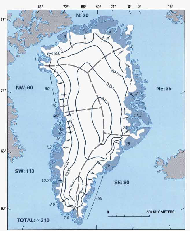
The generalized calving output of each section of the ice sheet (Figure 4, below) indicates the volume flux by quadrant and by glacier in some cases. 

Figure 4. Generalized calving output by quadrant, in cubic kilometers per year water equivalent based on the assumption of an equilibrium state. The contours indicate elevation in meters. (USGS Satellite Image Atlas of Greenland)

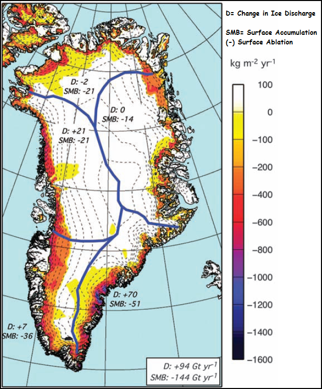
The northern quadrant is one of the largest in terms of the ice sheet perimeter, but the calving output is the lowest at 20 km³.  The northeast quadrant at 35 km³ is the second lowest.  The highest are the southwest and southeast quadrants at 113 and 80 km³, respectively.  The difference is the result of higher accumulation rates.   If we look at more recent work, which examines the changes in volume discharge and surface mass balance, we see the greatest discharge changes and surface loss are in the southeast. 

Figure 5. Higher calving flux indicates higher velocities (Van Den Broecke et al., 2009). D denotes change in ice discharge while SMB denotes the net surface mass balance (accumulation minus ablation).

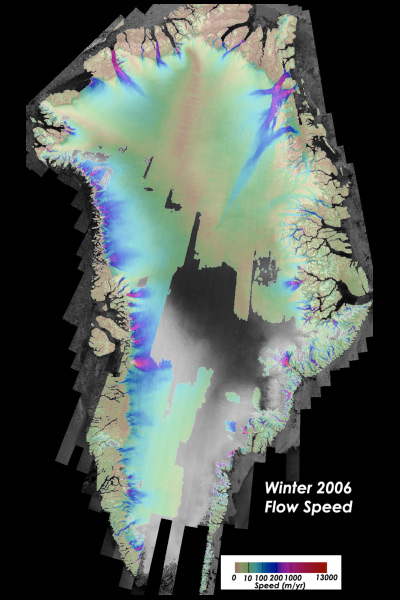
Figure 6. Ice flow speed in Greenland (color) for winter 2006 derived from synthetic aperture radar (SAR) imagery (gray scale image derived from NASA funded research). Because of the large range of speeds (1-13,000 m/yr), a log color scale is used (Ian Joughlin, Big Ice).

Hence the above velocity map of the glacier will indicate higher average velocities in the quadrants with the highest calving volume flux.  This map indicates relatively low flow rates of less than 10 m/year inland, with particular bands of fast flow that extend well into the ice sheet and feed outlet glaciers.  The variation in flow and accumulation rates indicates the problem of lumping the glaciers into one category. 

Climate change has led to an observed increase in surface melting, surface accumulation, increased discharge and overall mass balance losses.  The very mechanism that establishes the basics of behavior of the GIS mass balance are changing (Zwally et al., 2011).

Greenland glaciers fall into at least 4 common types, each with its own unique sensitivity to sea surface temperature, surface melting, meltwater lubrication, calving changes, etc.

Type 1: Northern, with Large Floating Termini

Northern glaciers with large floating termini (Petermann, Ryder, Steensby, Zachariae, Academy, etc).  Each of these is a marine terminating outlet glacier that has an extensive floating ice shelf.  The large ice shelves can exist in part due to the lower surface melt rates and the lower flow rates of the glacier.  Petermann Glacier is the fastest with a flow speed of 1,000 m/year at the grounding line.  This is much less than the average outlet glacier speed along the west coast.  The large floating ice shelves are susceptible to bottom melting but, except for Petermann Glacier, we have no observations of the process or that more warm water is penetrating under these ice shelves.  Rignot and Steffen (2008) found that at Petermann Glacier 80% of the ice loss into the ocean was from basal melting of the floating tongue.  If the ice shelves are removed, the feeding glacier is less buttressed and will accelerate for a period and draw down its surface profile.  The recent ice area lost by Petermann, Academy and Zachariae Ice Stream indicate these glaciers are being impacted by the increased melting at the surface and likely the base of the ice shelf for Petermann Glacier at least. 

Examination of how far the high velocities extend inland in Figure 6 indicates that it is only Zachariae and Petermann that tap far into the ice sheet.  This northern area has low accumulation rates, and a shorter less intense melt season.  The early onset of melting and lack of accumulation in 2010 led to an early exposure of the ablation zone on these glaciers. 

This is their sensitivity Achilles Heel:  relatively little increases in melt can expand the ablation zone appreciably given the low surface slopes and low accumulation rates.   Based on the velocity map, it is the Zachariae that is likely the only of this group that would be comparable to a bank that is too big to fail as its increased velocity band extends well into the ice sheet. 

Figure 7. Ice flow speed for Zachariae Glacier (Joughlin et al., 2010).

Type 2: Inland-terminating

Glaciers with inland termini lacking any calving (Sukkertoppen, Frederickshaab, Russell, etc.). Between the fast flowing marine terminating outlet glaciers, the ice sheet particularly in the southwest quadrant has numerous glaciers that terminate on land or in small lakes.  The velocity of these glaciers reaches a maximum of 1-2 meters/day.  Each terminates on land because total ablation over the glacier equals total accumulation at the terminus.  These glaciers are more like a typical alpine glacier and are susceptible to the forces that tend to cause alpine glaciers to experience peak flow during spring and early summer.  Those forces are the delivery of meltwater to the base of the glacier, when a basal conduit system is poorly developed.  This leads to high basal water pressure, which enhances sliding.  As the conduit system develops the basal water pressure declines as does sliding, even with more water.

Figure 8. Inland terminating glaciers (Sundal et al., 2011).

This is what has been recently reported to be the case by Sundal et al. (2011).  The meltwater lubrication mechanism is real, but as observed is limited both in time and area impacted.  It is likely that, as on alpine glaciers, the seasonal speedup is offset by a greater slowdown late in the melt season.  Most observed acceleration due to high meltwater input has been on the order of several weeks, leading to a 10-20% flow increase for that period.  The role of supraglacial lakes in this has been a point of emphasis; Luthje et al. (2006) noted that the area covered by supraglacial lakes was independent of the summer melt rate but controlled by topography.  This led Luthje et al. to conclude that  the area covered by supraglacial lakes will remain constant even in a warmer climate.  This suggests that the enhancement of flow by the drainage of such lakes would be limited.

The land terminating glaciers such as Sukkertoppen, Russell and Mittivakkat are retreating significantly in response to global warming.   This is an indication of negative mass balance. The latter glacier in southeast Greenland has retreated 1,200 meters since 1931 (Mernhild et al., 2011).  The Mernhild study identified this slow rate compared to the outlet glaciers and, based on mass balance observations, that the current surface mass balance can only support a glacier at most one-third its current size.   This indicates the slow but inexorable sensitivity of the non-calving glacier to surface mass balance change.  Moon and Joughin (2008) observed that the retreat of the land terminating glaciers was relatively minor from 1992 to 2007, averaging 5 m/year or less.  These glaciers are the equivalent in our banking system to the local banks:  there are many and they are sensitive, but the changes in a single one is not important. 

Type 3: Marine-terminating

Fast flowing marine terminating outlet glaciers of western and southeast Greenland (Rinks, Umiamako, Helheim, Jakobshavn, Epiq Sermia, etc.).  These are the glaciers that drain the greatest area of the ice sheet and deliver the greatest volume to the oceans via calving.  The flux from many of the larger glaciers is over 10 km³/year (DMI).  Each of these glaciers is fast-flowing at the terminus; the fast flow section extends inland into the ice sheet up a sub-glacial trough.  The outlet glaciers act like a drain capturing ice from a larger area of the ice sheet than their narrow terminus would suggest.  

Figure 9. Marine-terminating glaciers (Thomas et al., 2009).

Pelto et al. (1989), in a paper on the equilibrium state of the Jakobshavn Glacier, showed that the terminus had not changed significantly in 30 years; its velocity had also been consistent.  Furthermore, it was observed that the velocity was consistent throughout the seasons.  This indicated that the glacier velocity was not being impacted by the meltwater pulse of summer. 

Bob Thomas (NASA, 2004) and Terry Hughes (University of Maine, 1986) developed the basic mechanism of flow for the glacier that has proven to be true.  The outlet glaciers have a balance of forces at the calving front.  The fjord walls, the fjord base and the water column impede flow.  The slope of the glacier, its upglacier velocity and the height of the calving face strive to increase flow.  If the glacier thins than there is less friction at the calving front from the fjord walls and the fjord base, leading to greater flow.  The enhanced flow leads to retreat and further thinning, resulting in the thinning and the acceleration spreading inland.  In 1990 it was not envisioned that acceleration would occur as soon as it has, yet that was the motivation for the research. 

Figure 10. Jakobshavn profile (Thomas et al., 2009).

In 2001, the acceleration of the Helheim, Jakobshavn and Kangerdlussaq Glaciers caught the attention of the world.  By 2007, acceleration had been noted at all 34 marine terminating outlet glaciers observed.

The acceleration was not significantly seasonal; Howat et al. (2010) noted a 15% seasonal component to the acceleration: it had spread inland and had led to retreat and thinning.  This demonstrated that the marine terminating glaciers were largely responding to a change in the balance of forces at the glacier front. 

Figure 11. Ice flow velocity as color over SAR amplitude imagery of Jakobshavn Isbræ in (a) February 1992 and (b) October 2000. In addition to color, speed is contoured with thin black lines at 1,000 m/yr intervals and with thin white lines at 200, 400, 600, and 800 m/yr. Note how the ice front has calved back several kilometers from 1992 to 2000. Further retreat in subsequent years caused the glaciers speed to increase to 12,600 m/yr near the front (Ian Joughlin, Big Ice).

The recent increases in outlet glacier discharge have always been coincident with floating tongue losses.   This causes reduced back pressure at the glacier front, letting up on the brakes; the resulting glacier thinning leads to less basal friction and further acceleration.  If the glacier front retreats into deeper water the process will continue and increase.  This is why understanding the basal slope changes inland of the calving fronts is crucial. Moon and Joughin (2008) observed the terminus change of 203 glaciers from 1992 to 2007 and noted a synchronous ice sheet wide retreat of tidewater outlet glaciers. The thinning could be due to increased surface melt, basal melt or most likely a combination of the two.  Moon and Joughin (2008) reported for the 2000-2006 period:

• In the southeast quadrant 35 glaciers retreated an average of 174 m/year
• In the eastern quadrant 21 glacier retreated an average of 106 m/year
• In the northwest 64 glaciers retreated an average of 118 m/year. 

Each quadrant’s retreat increased markedly after 2000.  The largest of this group are comparable to the banks that are too big for our banking system to allow them to fail:  they drain a substantial portion of the entire ice sheet and reach so far into the ice sheet that their behavior can impact that of other adjacent glaciers.

Type 4: Marine-terminating in Shallow Water

Marine terminating glaciers outlet glaciers in shallower water (Humboldt, Cornell, Steenstrup, etc.).  These glaciers do have calving termini but lack the large fast flowing feeder tongues extending into the glacier.  This is because there is not a topographic low under the ice sheet that funnels the flow.  Humboldt Glacier is the widest front of any Greenland glacier, wider even than Petermann Glacier. 

Figure 12. Humboldt profile (Thomas et al., 2009).

However, the velocity on average is low at 100 m/year, and the base of the glacier is quite high.  This makes it difficult for a large calving retreat of the glacier to occur and extend inland.  Humboldt Glacier is retreating but, as the velocity profile indicates, the glacier, despite its size, does not tap dynamically into the center of the ice sheet.  These glaciers are substantial, but their failure (though significant for sea level) would not destabilize the ice sheet as a whole.

 Greenland Ice Sheet outlet glaciers: Zebras no more

 Overall in Greenland, the rate of area loss in marine-terminating glaciers during the 2010 melt season (419 km²) was 3.4 times that of the previous 8 years. There is now clear evidence that the ice area loss rate of the past decade (averaging 120 km²/year) is greater than loss rates pre-2000.  The exceptional extension of the ablation season in 2010 in southern Greenland indicates the vulnerability of these areas to expanded melt regions (Box et al., 2010). 

The amazing aspect of Greenland glaciers is that (despite the specific variation in type, location specific fjord configuration, etc.) their response has been as uniform and synchronous to global warming as has been observed.  If this warming of the world persists long enough, the  ice “banks” of Greenland will begin to fail.  Those with the greatest reserves on their asset sheets and the fastest turnover, and thus having the greatest potential contributions to sea level rise over time, are:

• In the north, Zachariae (and to a lesser extent, Petermann)
• The fast flowing marine terminating outlet glaciers of western and southeast Greenland (Rinks, Umiamako, Helheim, Jakobshavn, Epiq Sermia and Kangerdlussaq)

---

Further Reading & Resources

1. Pelto et al. (1989)
2. Luthje et al. (2006)
3. Moon and Joughin (2008)
4. Rignot and Steffen (2008)
5. Thomas et al. (2009)
6. Van Den Broecke et al. (2009)
7. Box et al. (2010)
8. Howat et al. (2010)
9. Joughlin et al. (2010)
10. Mernhild et al. (2011)
11. Sundal et al. (2011)
12. Zwally et al. (2011)
13. The USGS Satellite Image Atlas of Greenland

http://www.skepticalscience.com/Variations_in_Greenland_Glaciers.html

RETREAT OF GREENLAND'S HELHEIM GLACIER

RETREAT OF GREENLAND'S HELHEIM GLACIER

Left: May 12, 2001. Middle: July 7, 2003. Right: June 19, 2005. Along the margin of the Greenland Ice Sheet, outlet glaciers flow as icy rivers through fjords and out to sea. These pictures show a fjord in which Helheim glacier (on the left) is crumbling into large and small icebergs (light blue, on the right). The glacier outlet ("calving front") held steady from the 1970s until about 2001, then began to retreat towards its source about 7.5 kilometers (4.7 miles) between 2001 and 2005. The glacier’s flow to the sea has also sped up.  Click to enlarge.

I.M. Howat et al., GRL 38, Mass balance of Greenland's three largest outlet glaciers, 2000–2010

Geophysical Research Letters, 38 (2011) L12501; doi: 10.1029/2011GL047565.


Mass balance of Greenland's three largest outlet glaciers, 2000–2010


Ian M. Howat (School of Earth Sciences, and the Byrd Polar Research Center, Ohio State University, Columbus, OH, USA), Yushin Ahn (Byrd Polar Research Center, Ohio State University, Columbus, OH, USA), Ian Joughin (Polar Science Center, Applied Physics Laboratory, University of Washington, Seattle, WA, USA), Michiel R. van den Broeke (Institute for Marine and Atmospheric Research, Utrecht University, Utrecht, Netherlands), Jan T. M. Lenaerts (Institute for Marine and Atmospheric Research, Utrecht University, Utrecht, Netherlands) and Ben Smith (Polar Science Center, Applied Physics Laboratory, University of Washington, Seattle, WA, USA)


Abstract

Acceleration of Greenland's three largest outlet glaciers, Helheim, Kangerdlugssuaq and Jakobshavn Isbræ, accounted for a substantial portion of the ice sheet's mass loss over the past decade. Rapid changes in their discharge, however, make their cumulative mass-change uncertain. We derive monthly mass balance rates and cumulative balance from discharge and surface mass balance (SMB) rates for these glaciers from 2000 through 2010. Despite the dramatic changes observed at Helheim, the glacier gained mass over the period, due primarily to the short-duration of acceleration and a likely longer-term positive balance. In contrast, Jakobshavn Isbræ lost an equivalent of over 11 times the average annual SMB and loss continues to accelerate. Kangerdlugssuaq lost over 7 times its annual average SMB, but loss has returned to the 2000 rate. These differences point to contrasts in the long-term evolution of these glaciers and the danger in basing predictions on extrapolations of recent changes.

Received 24 March 2011; accepted 7 May 2011; published 18 June 2011


Howat, I. M., Y. Ahn, I. Joughin, M. R. van den Broeke, J. T. M. Lenaerts, and B. Smith. 2011. Mass balance of Greenland's three largest outlet glaciers, 2000–2010. Geophys. Res. Lett. 38, L12501, doi: 10.1029/2011GL047565.


http://www.agu.org/pubs/crossref/2011/2011GL047565.shtml

"Committed sea-level rise for the next century from Greenland ice sheet dynamics during the past decade" by S. F. Price, A. J. Payne, I. M. Howat & B. E. Smith, PNAS, May 16, 2011

Proceedings of the National Academy of Sciences, published online before print May 16, 2011; doi: 10.1073/pnas.1017313108

Committed sea-level rise for the next century from Greenland ice sheet dynamics during the past decade

1. Stephen F. Price^a,*, 
2. Antony J. Payne^b, 
3. Ian M. Howat^c, and 
4. Benjamin E. Smith^d

+Author Affiliations

1. ^aFluid Dynamics and Solid Mechanics Group, Los Alamos National Laboratory, T3 MS B216, Los Alamos, NM 87545;
2. ^bBristol Glaciology Centre, University of Bristol, University Road, Clifton, Bristol BS8 1SS, United Kingdom;
3. ^cSchool of Earth Sciences, Ohio State University, 125 South Oval Mall, Columbus, OH 43210; and
4. ^dPolar Science Center, Applied Physics Laboratory, University of Washington, Box 35560, Seattle, WA 98105

1. Edited by Hans-Joachim Schellnhuber, Potsdam Institute for Climate Impact Research, Potsdam, Germany, and approved April 19, 2011 (received for review November 22, 2010)

Abstract

We use a three-dimensional, higher-order ice flow model and a realistic initial condition to simulate dynamic perturbations to the Greenland ice sheet during the last decade and to assess their contribution to sea level by 2100. Starting from our initial condition, we apply a time series of observationally constrained dynamic perturbations at the marine termini of Greenland’s three largest outlet glaciers, Jakobshavn Isbræ, Helheim Glacier, and Kangerdlugssuaq Glacier. The initial and long-term diffusive thinning within each glacier catchment is then integrated spatially and temporally to calculate a minimum sea-level contribution of approximately 1 ± 0.4 mm from these three glaciers by 2100. Based on scaling arguments, we extend our modeling to all of Greenland and estimate a minimum dynamic sea-level contribution of approximately 6 ± 2 mm by 2100. This estimate of committed sea-level rise is a minimum because it ignores mass loss due to future changes in ice sheet dynamics or surface mass balance. Importantly, > 75% of this value is from the long-term, diffusive response of the ice sheet, suggesting that the majority of sea-level rise from Greenland dynamics during the past decade is yet to come. Assuming similar and recurring forcing in future decades and a self-similar ice dynamical response, we estimate an upper bound of 45 mm of sea-level rise from Greenland dynamics by 2100. These estimates are constrained by recent observations of dynamic mass loss in Greenland and by realistic model behavior that accounts for both the long-term cumulative mass loss and its decay following episodic boundary forcing.

• ice sheet modeling
 
• climate change

• *Correspondence e-mail: sprice@lanl.gov
• http://www.pnas.org/content/early/2011/05/09/1017313108.abstract